Modeling Retinal Damage for Threshold Prediction and Probabilistic Risk Assessment

Summary

A modeling approach for laser-induced thermal damage to the human eye is presented. It aims to improve the evaluation of laser-based hazards by providing a means of calculating the damage for a specific irradiation scenario.

Abstract

With the increasing number of laser applications in medicine, defense, and technology, both intentional and accidental exposure of the human eye to laser sources has become a major concern. Model-based prediction of retinal damage thresholds could enable more scenario-specific laser safety assessment, especially for laser parameters not covered by experimental data. Ideally, such models would allow the calculation of ED50 (effective dose at which the likelihood of damage is 50%) values based —among other factors — on wavelength, pulse duration, and spot shape. This requires a detailed understanding and modeling of all damage regimes to reflect the dependency between the key parameters and the dominant damage mechanism.

This work discusses the status of this approach (validated here for the thermal regime, or simply "in the thermal damage regime"); critical aspects that could block its success are highlighted, and potential benefits are outlined. These range from improved accuracy of laser exposure limits in eye safety standards to optimized dosimetry in retinal laser surgery to probabilistic risk assessment for the use of lasers in outdoor environments.

Introduction

This work describes the development and validation of a physiologically detailed thermal damage model of the human eye. Within the thermal injury regime, the model predicts retinal temperature evolution and injury thresholds using an Arrhenius damage formulation (compare explanation in the photothermal damage section). Representative applications cover all situations in which the prediction of ocular temperatures and damage is of interest. This includes, e.g., evaluating damage thresholds for scanned retinal irradiation, understanding the effect of pulse-train additivity on damage thresholds, and comparing computed thresholds with safety limits from the laser safety standard. Outside the thermal regime, current modeling approaches under consideration are presented, and a roadmap is provided toward extending the framework to additional damage mechanisms.

The work presented here concerns the modeling and, therefore, the prediction of retinal damage caused by laser irradiation. While a critical dose could, in theory, always be determined by experiments with animal retinas similar to human retinae, there is a strong need to predict the damage without performing experiments. The laser parameter space of variation (wavelengths, pulse durations, and repetition rates) is vast, implying a prohibitively large number of animal experiments for each new parameter set. Additionally, for long irradiation times, retinal blood flow must be considered as well, which would require in vivo experiments. Consequently, modeling the interaction of the laser with the eye seems to be the only realistic way forward.

The need for a detailed understanding of damage mechanisms and, therefore, damage thresholds (which could be used as ED50 surrogates) is also linked to the situation of the eye safety standard (IEC 60825 or ANSI Z136.1). Because the standard must address the full range of wavelengths, pulse durations, repetition patterns, and spot sizes, it necessarily incorporates simplifying assumptions, interpolations, and conservative safety factors to account for uncertainty. As only a limited number of ED50 values—primarily derived from non-human primate studies—are available, interpolation is required to establish comprehensive MPE (maximum permissible exposure) limits. Although this approach provides broad and practical applicability, a framework grounded in a detailed mechanistic understanding and modeling of damage processes offers clear advantages in terms of physical transparency, scenario-specific accuracy, and applicability without detailed knowledge of the laser safety standard.

For example, pulsed and scanning lasers are evaluated as pulsed sources, although retinal scanning introduces additional temporal and spatial effects. The appropriate treatment of scanning in the derivation of safety limits has been the subject of ongoing discussion within the community over the past decade. Even with regular updates to reflect technological advances, it is not feasible for the standard to cover every complex configuration of new laser systems with new sets of parameters without simplifications and conservative safety factors. Consequently, room for interpretation remains, which may lead to inconsistencies or errors in safety evaluation.

A physics-based modeling approach could substantially reduce reliance on interpolation and conservative margins and extend the standard's applicability to complex scenarios. Because the development and validation of such models are directly linked to a deeper understanding of the underlying damage mechanisms, the resulting insights could also support a more transparent and physically grounded derivation of MPE values from existing ED50 data.

In the long term, eye safety assessment could be streamlined through an integrated, plug-and-play modeling framework. Such a tool could be supplied either with the relevant system parameters or directly with an optical design file (e.g., a Zemax model), which is typically available during product development, thereby enabling consistent and scenario-specific safety evaluation¹.

Another field of application is the growing field of high-energy lasers (HEL), e.g., to counteract drones. Here, the difficulty mostly resides in the laser reflections from targets, especially metallic targets, that can change rapidly and randomly and constitute a hazard to military personnel and civilians^2,3. This random non-deterministic situation requires an adequate evaluation mechanism – usually a probabilistic approach is used. This approach creates statements about the occurrence of certain irradiation situations (intensity, exposure time, wavelength), which still must be translated into a likelihood of damage. Here, the damage modeling discussed in this work can close the gap by translating probabilistic scenarios into likelihoods of damage.

Understanding the principles of damage mechanisms in detail and mimicking these in a software model is a straightforward way to determine damage thresholds instead of performing experiments. Depending on the pulse duration, retinal damage occurs via different laser-tissue interaction mechanisms (Figure 1)^4,5,6,7:

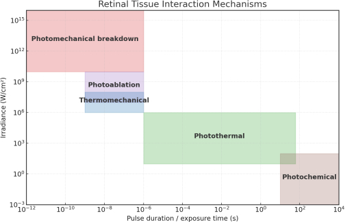
Figure 1: Overview of the damage mechanisms. The type of damage mechanism depends on the exposure time and irradiance. It ranges from photomechanical damage following from very high irradiance at short pulse durations to photochemical damage due to low irradiance for long time durations. Please click here to view a larger version of this figure.

Photomechanical breakdown (10^-12–10^-6 s, 10¹⁰–10¹⁶ W/cm²):
Photodisruption: At ultrashort to nanosecond pulse durations and very high irradiances, nonlinear absorption initiates optical breakdown. A dense plasma of free electrons and ions forms, expanding explosively and generating strong shock waves. The process, called photodisruption, mechanically tears tissue apart with minimal bulk heating and creates sharply defined lesions even in weakly absorbing areas^4,8,9,10.

Plasma-induced ablation: In the ns–µs range at very high irradiance, plasma again dominates. Here, tissue removal is driven not just by shock waves but also by plasma expansion and explosive ablation. The mechanism is known as plasma-induced ablation and produces significant material ejection^4,11.

Photoablation (≈ 10^⁻9–10⁻⁶ s; ≈ 10⁷–10¹⁰ W/cm²):
For pulse durations above the nanosecond and below the microsecond range, photoablation occurs. In this process, molecular bonds are directly broken by the irradiation. This method is, for example, used to correct refractive errors of the eye by reshaping the cornea (the so-called LASIK method). Typically, photoablative procedures are applied in a power range where plasma formation has not yet occurred^4,11.

Thermomechanical damage (≈ 10^-9 – 10^-6 s; ≈ 10⁶ – 10⁸ W/cm²):
In pigmented ocular tissues, strong absorption by melanosomes in the ns–µs range can cause rapid superheating. When the melanosome surface reaches ≈ 150 °C, microbubbles nucleate^12,13. Their expansion and collapse generate mechanical stress waves that damage the retinal pigment epithelium (RPE). This thermomechanical mechanism bridges the gap between photoablation and thermal injury: it is not plasma-driven, but involves mechanical transients coupled to localized heating. Thresholds depend on melanosome size, shape, orientation, and local illumination^4,11.

Photothermal damage (≈ 1 µs– 60 s; ≈ 10– 10⁶ W/cm²):
From microseconds up to seconds, tissue heating dominates. Energy deposition raises temperature, leading first to protein denaturation and, with higher exposures, coagulative necrosis and carbonization. Literature bounds differ: Niemz⁴ cites 1 µs – 60 s, Zuclich¹⁴ 10 µs–60 s. Approximate reciprocity with radiant exposure (~1–1000 J/cm²) holds, with deviations for very short pulses (limited heat diffusion) and very long pulses (enhanced cooling by perfusion)^4,6,15.

The modeling of the thermal damage in the presented work is based on the Arrhenius integral, which is defined as:

   (1)

With τ denoting the exposure time, E_a the activation energy, R the universal gas constant, T the temperature during exposure, and A a pre-exponential scaling factor, the parameters applied in this study are A = 1.3 × 10⁹⁹ s⁻¹ and E = 628 kJ/mol¹⁵. A condition of Ω = 1 is taken to indicate the onset of tissue damage. For a comprehensive discussion of the underlying model, refer to a previous publication⁴.

Photochemical damage (≈ 10 s – 10⁴ s; ≈ 10⁻³ – 10² W/cm²):
For long exposures at low irradiances, cumulative photochemical reactions dominate - such as photopigment bleaching or reactive oxygen species (ROS)-mediated pathways. They occur at exposure durations above 10 s⁶ (or above 1 s⁴). Thus, there exists an intermediate range in which both thermal and photochemical damage can occur simultaneously¹⁶. Chronic low-level blue-light hazard is a typical example.

Protocol

Section 1 describes the general steps necessary for model building, as they can be performed with a variety of software options. Section 2 gives these instructions for the specific and exemplary case where Altair Hypermesh (finite element modeling and analysis [FEA] software) and Ansys Fluent (fluid simulation software) are used. In addition, a supplementary file (Supplementary File 1^{17,18,19,20,21,22,23,24,25,26,27,28,29,30,31,32,33,34,35,36,37,38,39,40,41,42,43,44,45}) is provided, which describes the modeling approach and gives theoretical background in a non-stepwise manner (Figure 1 - Figure 5,  Table 1 - Table 3).

1. Implementation of the modeling approach – General procedural steps

1. Create a 3D model according to the geometry as described above.
   1. Within this work, create the geometry in a 3D mechanical computer-aided design software (Version 16) according to the parameters described in Supplementary File 1.
2. Create the volume mesh according to the properties and extensions of all parts of the eye, according to Supplementary File 1.
   1. Carry out meshing and post-processing with FEA analysis software (Version 11) and computer-aided engineering (CAE) analysis software (Version 11). The model consists of 761,766 tetrahedral elements. The mesh cells have dimensions between 37 µm and 491 µm.
      NOTE: A coarser meshing would result in calculational errors/deviations. A higher number of cells is always possible, but it would increase computational time. This mesh proved to be size-independent, as further refinement of the element size resulted in negligible differences in the calculations.
   2. To maintain reasonable computation times, use this mesh and adopt only if specific regions require a finer resolution. Accordingly, remesh the retina with a minimum feature size of 5 µm to enable absorption within the RPE layer, as required and explained later in the protocol.
      NOTE: Figure 2 shows an exemplary image of the mesh with a hidden vitreous to make the retina visible.
3. Integrate boundary conditions.
   1. At the sclera, use a conduction-only boundary coefficient h_scl = 20 W/m²K and a corneal value h'_corn,1 = 14.21 W/m²K of as derived above in detail. Use these values to define the boundary conditions of the surface representing the sclera and cornea, respectively.
4. Implement the blood flow.
   NOTE: This field supplies flow direction and magnitude in every mesh cell and adds advection to the energy equation.
   1. Follow the construction steps as mentioned below:
      1. Specify physiological inlets/outlets—anterior inflow from the major arterial circle of the iris and posterior inflow from the short ciliary arteries, with venous drainage via the vortex veins.
      2. Compute the resulting flow field.
      3. Rescale all local speeds to a uniform 5 mm  (per Peyman⁴⁵) while preserving directions, implemented via a fluid simulation software user-defined function (UDF). The outcome is a directionally correct velocity field of constant magnitude across the choroid.
5. Calculate the temperature distribution.
   1. Begin the temperature calculation with the definition of the time-dependent positions and shapes of the laser beam. To obtain these time-varying positions on the retina (or within the eye more generally), use a raytracing software model of the eye in parallel with the thermodynamical model.
      NOTE: Based on the raytracing software modeling of the laser system under evaluation, this approach provides the temporal evolution of the laser spot positions and shapes. This is not explained in detail in this work for the sake of accessibility, but is described previously^1,18.
   2. Map the calculated spot-positions and shapes onto the corresponding sections of mesh cells over time, which are then assigned the respective laser power.
   3. Import these data into the fluid simulation software via a UDF, which processes them cyclically. The UDF identifies the relevant mesh cells and introduces an energy source term according to the specified laser power for the corresponding irradiation time. Consider both continuous-wave (cw) and pulsed irradiation, as well as static or time-dependent beam movements.
   4. For each position, calculate the absorbed energy using the absorption coefficient at the given laser wavelength and assign it to the affected mesh cells, which are heated in parallel.
      NOTE: As an example, for irradiation at a wavelength of 532 nm, 51% absorption occurs in the RPE with a thickness of 5 µm⁷, as shown in Figure 3. No absorption occurs within Bruch's membrane^7,46. The remaining laser energy decreases in the choroid, assumed to be 100 µm thick with an absorption coefficient⁷ of α_Ch = 270 cm^-1, according to the Lambert-Beer law. The UDF calculates the absorbed energy across the thickness of each mesh cell and assigns this value to the cell. For the transmission from cornea to retina, a value of 20 % is applied⁷. A change in laser wavelength is easily accommodated by simply adapting the absorption coefficient and the transmission from cornea to retina.
   5. In addition, define the duration of a single time step, since the spot-shape data (from the raytracing model or defined directly in the UDF if it is known without the raytracing model) only describes the irradiation sequence without a temporal scale.
   6. To accelerate the calculation, group all intervals without irradiation together and assign a correspondingly larger time step, as no fine temporal resolution is required there.
      NOTE: After these settings are applied, the solver can compute the temporal thermal response of the eye. Since the present model only requires heat conduction and blood flow to be considered, the solver is restricted to solving the corresponding differential equations. Refer to Supplementary File 2 for exemplary user-defined functions.
6. Calculate the damages.
   1. To derive a damage threshold based on the thermal response, extract the calculated temperature values from the Fluent result file using a C++-based tool (see^1,18 for details and code listings).
   2. Following the Arrhenius integral approach, calculate the Arrhenius values of the individual mesh cells from these temperatures and store them in a format compatible with the post-processing software. This enables convenient switching between temperature values and damage probabilities during analysis.
   3. Finally, obtain a binary damage outcome (yes/no) for each mesh cell. Determine the yes/no classification by a threshold value of 1 for the Arrhenius integral⁴. Identify this damage threshold iteratively by testing different input powers for a fixed irradiation duration.
7. Set solver-timestep size.
   1. Use the fluid simulation software (Version 14.5) as the solver, employing the finite volume method. The step size shall satisfy the Courant-Friedrichs-Lewy condition, which describes the ratio to the size of the mesh cells in order to create stable simulation conditions.
   2. Also, reduce the step size step-by-step until the result becomes invariant to the step size. E.g., for calculations with up to 10 s time steps of 1 ms and 100 ms, the temperature changes were found to be <1%.

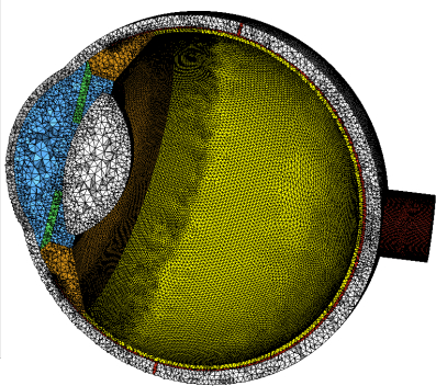
Figure 2: Section cut through mesh (vitreous humor masked out). The figure shows the sclera (white), the choroid (red), the retina (yellow), the lens (white), the iris (green), and the aqueous humor (blue)¹⁸. Please click here to view a larger version of this figure.

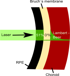
Figure 3: Absorption characteristics at the ocular fundus. Within the RPE, 51% of the 532 nm laser radiation is absorbed; no absorption occurs in Bruch's membrane, and the choroid is modeled according to Lambert-Beer behavior¹⁸. Please click here to view a larger version of this figure.

2. Illustrative example – Specific steps

1. Create a 3D model according to the geometry as described above.
   NOTE: The 3D model is built by creating objects for all elements listed in Supplementary Table 1. As an example, these steps will lead to the sclera.
   1. Create a new part file (.ipt).
   2. Start a 2D sketch on the XY-plane.
   3. Draw a horizontal construction line (this will be the rotation axis).
   4. Draw an arc with a radius of 12 mm for the outer surface.
   5. At the center (posterior pole), create a point 0.99 mm inward from the outer arc.
   6. From this point, sketch the inner surface curve.
   7. At the limbus, set the distance between the inner and outer surface to 0.75 mm.
   8. Connect inner and outer curves at the edge to form a closed profile.
   9. Select 3D Model > Revolve.
   10. Choose Surface and confirm.
2. Create the volume mesh.
   NOTE: The mesh is created based on the 3D object. This is an example for meshing:
   1. Import the 3D model created in the 3D mechanical computer-aided design software.
   2. Click on the surface of the object to mesh, e.g., the sclera.
   3. Mesh the surfaces first – click Mesh in this interface, which appears once the surface is clicked upon. Select surfs in the interface and select automatic adaptive meshing.
   4. The 3D mesh (defining the object) is based on the surface meshes. To create, select the surfaces and click from the top left menu: Mesh > Create > Solid Map Mesh.
   5. Now, an interface appears. Click mesh.
3. Integrate boundary conditions.
   NOTE: Boundary conditions have to be defined for the sclera and cornea, since these surfaces are in contact with the surrounding world. This example is for the sclera:
   1. Go to Analysis from the top menu > BCs > Create > Constraints (or Loads).
   2. Select the entity type surfaces and pick the sclera from the menu.
   3. In the same panel, locate the value input fields and enter the value directly in the magnitude field.
   4. Click create to assign the boundary condition.
4. Implement the blood flow.
   1. Define surfaces for - anterior inflow (major arterial circle of iris), posterior inflow (short ciliary arteries), and outflow (vortex veins).
   2. Assign boundary conditions for these surfaces.
   3. Click on Analysis > BCs > Create > Loads.
   4. Select inlet surfaces > assign velocity direction vectors (approximate physiological directions).
   5. Select outlet surfaces > assign pressure outlet (or zero constraint depending on solver setup).
   6. Export model to the fluid simulation software – this is where the length of the flow vector will be adapted.
   7. Use the ScaleVelocity UDF from the annex within the fluid simulation software to adapt the length of the vector (UDF is a standard format to be loaded into the fluid simulation software).
5. Calculate the temperature distribution (Set Solver).
   NOTE: Use the fluid simulation software to calculate the temperatures like the following and save it in a file format readable by the CAE analysis software.
   1. Click File > Read > Mesh > Select mesh > Mesh > Check.
   2. Click General > Solver: Pressure-Based > Time: Transient.
   3. Click Models > Energy > Enable > OK.
   4. Click Materials > define ρ, p, kρ > Cell Zone Conditions > assign materials to all regions.
   5. Click Boundary Conditions > define thermal BCs (cornea, sclera, environment).
   6. Click Solution Initialization > Initialize.
   7. Click Run Calculation > set Time Step Size + Number of Time Steps + Iterations per step.
   8. Click Run Calculation > Calculate.
   9. Click File > Export > Solution Data… > File Type: Ensight Gold > select Temperature > select zones > Write.
6. Calculate the damage.
   1. Execute the AddingArrhenius.exe (Supplementary File 3 and Supplementary File 4) from the same folder as the FEA analysis software files containing the temperatures. It contains a simple calculation of the Arrhenius integral based on the temperatures stored in the FEA analysis software files.

Results

This section shows the verification and validation of the presented model first. Afterward, three exemplary applications are demonstrated.

Verification and validation
In this section, the presented model is first verified by comparison with established thermo-physiological eye models^{19,27,28,30,32} to ensure cons...

Discussion

Within the protocol, there are no critical steps with respect to the creation of the model. Critical is the selection of the mesh size and type in combination with the time step size. A modification of the modeling technique is relevant with respect to employing other scanning patterns on the retina. The model itself shall not be modified. The technique is limited to the damage regimes as explained in the respective section. The significance lies in the possibility of damage prediction without animal experiments. One of ...

Materials

List of materials used in this article

Name	Company	Catalog Number	Comments
Altair Hypermesh 11.0	Altair Engineering Inc.	Version 11	Mesh creation and display; finite element modeling and analysis [FEA] software
Ansys Fluent 14.5	Ansys Inc.	Version 14.5	Thermodynamical solver; fluid simulation software
Autodesk Inventor	Autodesk	Version 16	3D mechanical computer-aided design software
Hyperview	Altair Engineering Inc.	Version 11	computer-aided engineering (CAE) analysis software
Optic Studio 13 (Zemax)	Zemax Development Corporation, today it is Ansys Inc.	Version 13	Raytracing Software
Optocon FOTEMP2	Optocon	https://comem.com/en/optocon/	Spectrometer; Temperature measurement of ocular tissue
Optocon TS2	Optocon	https://comem.com/en/optocon/	Measurement probe; Temperature measurement of ocular tissue