Patient-Specific Electric Field Simulation In Spinal Metastasis Electrochemotherapy

Summary

This protocol describes a complete, reproducible workflow for patient-specific electric-field simulation and validation of electrochemotherapy (ECT) for spinal metastasis. The workflow integrates multimodal imaging, semi-automatic and manual segmentation, tissue conductivity modeling, linear finite-element electric-field simulation, and experimental validation via post-procedure MRI-based necrosis overlap analysis.

Abstract

Electrochemotherapy (ECT) combines the administration of cytotoxic agents with high-voltage electric pulses that transiently permeabilize tumor cell membranes and enhance intracellular drug uptake. This minimally invasive, nonthermal technique is particularly suitable for tumors located near critical structures, where surgery, radiotherapy, or percutaneous thermal ablation may be limited. In the spine, ECT can provide pain relief, neural decompression, and local tumor control while preserving neural structures. However, its implementation remains challenging due to complex vertebral anatomy, limited understanding of electric field distribution, the absence of dedicated planning tools, and the risk of neural injury. This protocol describes a reproducible workflow for patient-specific electric field simulation in spinal ECT. Multimodal imaging combining CT and MRI enables reconstruction of tumoral, vertebral, neural, and soft-tissue anatomy using semi-automatic and manual segmentations performed within the open-source 3D Slicer platform. Tissue conductivities are assigned according to the IT’IS database, and linear finite-element simulations (constant conductivity) are performed with AI4DEEP, a dedicated 3D Slicer module, to compute 3D electric field maps across multiple isodose thresholds. Follow-up contrast-enhanced MRI is used for validation through Dice similarity coefficients comparing simulated isoelectric field volumes with post-ECT necrotic tumoral areas. Qualitative comparison of simulated electric field maps, follow-up MRI, and clinical outcomes was performed by expert interventional radiologists to evaluate the ability of the software to predict undertreated and overtreated regions. Nine ECT procedures were processed to assess the workflow. The highest concordance between simulated electric field and post-ECT necrosis was observed in the 160–200 V/cm range in this specific clinical and numerical setting. The workflow also identified regions of insufficient or excessive treatment, consistent with clinical and imaging follow-up. The described workflow lays the groundwork for reproducible ECT planning, supporting optimized electrode placement and parameter adjustment to improve safety and efficacy in complex spinal ECT procedures.

Introduction

Spinal metastatic epiduritis is frequent because the spine is the predominant site of skeletal metastases, accounting for up to 50% of all bone localizations^1,2. Clinical presentation typically includes severe pain with marked impairment of quality of life, followed by rapidly progressive neurological deficits that may end in paraplegia or tetraplegia, depending on the level of involvement^3,4. Radiotherapy is the standard of care for metastatic epidural spinal cord compression, while decompressive and stabilizing surgery benefits selected patients with adequate performance status and expected survival^5,6. Stereotactic ablative radiotherapy can improve local control in selected cases but is limited by spinal cord tolerance and planning complexity⁷. Local recurrence or progression after radiotherapy is frequent, and re-irradiation is limited by cumulative dose constraints, often resulting in therapeutic dead-ends for patients with persistent pain or progressive neurological compromise^6,7. In this context, a local nonthermal technique capable of achieving pain relief, decompression, and tumor control near critical neural structures is needed.

Electrochemotherapy (ECT) combines the administration of cytotoxic agents, most commonly bleomycin, with short high-voltage electric pulses that transiently increase plasma membrane permeability and enhance intracellular drug uptake^8,9. ECT is minimally invasive, nonthermal, and relatively tumor-selective, and has shown encouraging results for cutaneous, subcutaneous, and deep-seated tumors located close to critical structures^10,11. A recent clinical series reported an MRI objective response rate of 77% at 1 month and 66.5% at 3 months after percutaneous spinal ECT for radiotherapy-resistant epidural spinal cord compression. Pain also decreased markedly, with the median Numeric Rating Scale pain score decreasing from 7 at baseline to 1 at 1 month. Irreversible neurological deficits still occurred in a subset of patients¹². These events highlight the central role of electric field distribution: small changes in electrode geometry or tissue properties can markedly alter the treated volume, exposing patients to both undertreatment and overtreatment^13,14. Numerical studies suggest that patient-specific modeling can optimize electrode placement and improve coverage of vertebral tumors while limiting exposure of neural structures^15,16.

Several research planning frameworks have been proposed for electroporation therapies, but routine clinical implementation remains limited by meshing/parameter requirements and computation time^{17,18,19,20,21}. Recent work by Sutter and Poignard supports a peri-procedural, imaging-driven simulation workflow compatible with clinical constraints and shows that incomplete electric-field isodose coverage accurately correlates with local failure after IRE^22,23. This protocol builds on the same simulation framework.

The aim of this article is therefore to provide a reproducible, patient-specific workflow for electric field modeling and validation in spinal ECT, based on real clinical imaging datasets and delivered electrode configurations. In its current form, this workflow is best suited for pre-procedural planning to optimize electrode positioning, as segmentation and model preparation times remain a limitation for routine intra-procedural adjustment. It is intended as a methodological framework rather than a hypothesis-driven efficacy study and is designed for interventional oncology and spine teams already performing or planning percutaneous CT-guided ECT in epidural metastases and other anatomically complex settings.

Protocol

This retrospective study was conducted in accordance with the institutional ethics committee (IRB 2025-566) and complied with applicable national regulations. All imaging data were anonymized prior to analysis, and the requirement for informed consent was waived because of the retrospective design and use of de-identified data. The equipment and the software used are listed in the Table of Materials.

1. Data import and scene preparation

1. Import all anonymized DICOM series into 3D Slicer (available at https://download.slicer.org/) and assign explicit names to each volume: “MRIp” (pre-procedural MRI), “CTi” (initial intra-procedural planning CT), “CTa” (intra-procedural CT with needles in place), and “MRIs” (post-procedural MRI).
2. Set “CTi” as the reference volume for all subsequent segmentations and registrations.
3. Create a new segmentation node in 3D Slicer and link it to “CTi” as the “source volume”.
4. Save the Slicer scene as a baseline project file to allow recovery and future modifications.
   NOTE: Voxel size standardization is not required and can be omitted if native image resolution is adequate.

2. Anatomical segmentation on initial CT (CTi)

1. Open the Segment Editor module and create a segment named “Cortical bone”. Use the “Threshold” tool on “CTi” to isolate high-density cortical bone, then refine the segment manually using Scissors or Paint tools if needed.
2. Create a segment named “Fat”. Use the Threshold tool to select low-density fat, for example, in the perirenal or subcutaneous space.
3. Create a segment named “Intervertebral disc”. Use the 3D Paint tool on axial, sagittal, and coronal views, and check Paint outside existing segments, ensuring that painting is restricted to empty voxels to avoid overwriting existing segments.
4. Create a segment named “Cancellous bone” for vertebral cancellous bone. Use the 3D Paint tool to fill the internal trabecular compartments, and check Paint outside existing segments as described above.
5. Create a segment named “Spinal cord”. Use the 3D paint tool to manually contour the cord on axial slices from above to below the treated levels.
6. Create a segment named “Cerebro-spinal fluid”. Use the 3D paint tool to fill the cerebrospinal fluid space surrounding the spinal cord within the thecal sac, also checking the Paint outside existing segments.
7. Create additional segments for cement, coils, or lungs if present. Use the Threshold tool to identify hyperdense cement or coils and hypodense lung parenchyma, followed by manual correction as needed.
8. Save the updated Slicer scene.
   NOTE: Background voxels not explicitly assigned to a segment are later treated as “muscle-like” tissue in AI4DEEP (default conductivity).

3. MRI fusion and tumor segmentation

1. Import the pre-procedural MRI volume “MRIp” into the Slicer scene.
2. Use the Transforms module to perform a rigid registration of “MRIp” onto “CTi”, using vertebral osseous landmarks at the treated level. Registration is guided by four predefined landmarks: the tip of the spinous process and the tip of one transverse process on the axial plane, and the tip of the spinous process and the anterior cortical margin of the vertebral body on the sagittal plane. Because the posterior vertebral cortex is often altered by lytic disease, it should not be used as the primary landmark.
3. Apply the transform to “MRIp” and visually assess co-registration in axial and sagittal planes. The target registration error (TRE) is defined as the mean in-plane distance, in millimeters, between the corresponding CT and MRI landmarks at the predefined axial and sagittal reference points. Accept the registration only if both visual alignment and TRE are less than 2.5 mm; otherwise, repeat the registration.
4. Create a new segment named “Tumor” and use the Paint tool on “MRIp” (or on “CTi” when the epiduritis is well seen) to manually delineate epidural and vertebral tumor involvement at baseline.
5. Apply optional smoothing to the “Tumor” segment to obtain a coherent 3D volume without gaps.
6. Save the updated Slicer scene.
   NOTE: One may pause the protocol here and resume later from this step.

4. CT with needle fusion and electrode definition in AI4DEEP

1. Import the intra-procedural CT with needles, “CTa”, into 3D Slicer.
2. Use the Transforms module to perform a rigid registration of “CTa” onto “CTi” using the same vertebral bony landmarks as above.
   NOTE: In this workflow, “CTi” and “CTa” are acquired under general anesthesia without patient mobilization between the initial scan and electrode placement, such that CT-to-CT alignment is usually already close to optimal and requires no manual adjustment. TRE is therefore not applicable. With bone window settings, the metallic artifacts generated by the electrodes do not hinder visualization of the vertebral landmarks used for registration.
3. Launch the AI4DEEP module and create one virtual needle for each electrode, starting from the active electrode tip.
4. Verify in axial, coronal, and sagittal views that each “Electrode_n” matches accurately with a single physical active tip.
   NOTE: The quality of overall anatomical structure and electrode segmentation, as well as correspondence with the physical electrodes, is externally validated by an expert interventional radiologist who was not involved in the segmentation process. If deemed unsatisfactory, the segmentation is revised accordingly.
5. Save the updated scene containing anatomical structures, tumor segmentation, and electrode geometry.
   NOTE: The exact active tip length is specified later in AI4DEEP during the ECT parameter configuration and does not need to be encoded at this stage.

5. Conductivity assignment in AI4DEEP

1. In the AI4DEEP interface, assign each anatomical segment to a corresponding tissue class with predefined electrical conductivity (for example: tumor, cortical bone, cancellous bone, cerebrospinal fluid, epidural fat, intervertebral disc, spinal cord, cement, lung) as shown in Table 1.
2. Set the default background tissue to “muscle” conductivity so that all non-segmented voxels are treated as muscle.
3. Confirm in the AI4DEEP summary panel that each segment is mapped to the expected tissue type and conductivity, then save the configuration.
   NOTE: Conductivity values are derived from the IT’IS database and used as fixed (linear) conductivities for all simulations²⁴.

6. Pulse and needle characteristics

1. In AI4DEEP, specify the active tip length for each electrode (for example, 20 mm, 30 mm, or 40 mm) according to the clinical procedure. Electrode diameter was 1.8 mm.
2. Enter the clinically applied electric field amplitude in V/cm (for example, 500 V/cm, 600 V/cm, or 1000 V/cm).
3. Define the electrode pairs that were activated during the treatment.
4. Let AI4DEEP compute the applied voltage for each electrode pair based on the inter-electrode distance, ensuring the requested voltage-to-distance ratio in V/cm is respected.
5. Set the number of pulses (8) and the pulse duration (100 µs) according to the clinical protocol.
6. Save the AI4DEEP configuration.
   NOTE: Voltage is entered as a voltage-to-distance ratio in V/cm; AI4DEEP automatically converts this value into an absolute voltage for each electrode pair.

7. Electric field simulation

1. In AI4DEEP, start the electrostatic field computation using the configured anatomy, conductivities, and electrode parameters.
2. Allow the software to automatically generate the geometrical configuration and solve the linear electrostatic potential using high-order unfitted finite difference methods on the medical image²⁵.
   NOTE: On a typical workstation (for example, Windows 11, 16 GB RAM), processing takes approximately 5 min per case.
3. Save the simulation output and the updated Slicer scene.
   NOTE: One may pause the protocol here after simulation and resume later for isodose analysis and validation.

8. Isodose visualization and tumor coverage

1. In AI4DEEP, select the option to generate electric field isosurfaces (isodose volumes) from the simulated field.
2. Select a range of isodose thresholds (for example, 50 V/cm, 100 V/cm, 120 V/cm, 140 V/cm, 160 V/cm, 180 V/cm, 200 V/cm, 220 V/cm, 240 V/cm, 260 V/cm, 300 V/cm, 400 V/cm, 500, and 600 V/cm) and generate the corresponding 3D isodose maps.
3. Display individual isodose maps in 3D view to observe the spatial field distribution, typically ranging from pale yellow at low field amplitudes to red at high field amplitudes as shown in Figure 1.
4. For each isodose, record the percentage of tumor coverage values automatically computed by AI4DEEP based on the overlap between the isodose volume and the “Tumor” segmentation.
5. Save all isodose segments or models and the tumor coverage values for subsequent analysis.

9. Post-procedural MRI selection, import, and necrosis segmentation

1. Follow-up MRIs were performed at 6 weeks after ECT and every 2 months thereafter. The MRI showing the largest necrotic volume or the best radiological response was selected for segmentation. This choice was made to account for the heterogeneous and delayed time to response after ECT, which may vary according to tumor histology and proliferation rate.
2. Import the post-treatment contrast-enhanced T1 fat-suppressed axial sequence centered on the treated levels “MRIs” into 3D Slicer.
3. Perform rigid registration of “MRIs” onto “CTi” using the same predefined vertebral landmarks as those used for pre-procedural MRI registration, and apply the transform. Registration accuracy is documented by calculating the TRE from these same reference landmarks with the same ≤2.5 mm threshold.
4. Create a new segment named “Tumor necrosis” and manually delineate the non-enhancing necrotic portion of the tumor on the post-ECT MRI, slice by slice.
5. When multiple follow-up MRIs are available, select the examination demonstrating the largest necrotic volume or best radiological response and use this dataset for segmentation.
6. Apply optional smoothing to “Tumor necrosis” to obtain a coherent, contiguous volume.
7. In cases of complete radiological response after ECT, the pre-treatment “Tumor” segment may be duplicated and renamed “Tumor necrosis” to reduce manual segmentation time. In 3D Slicer, use the Segmentations module, select “Copy/move segments”, duplicate the “Tumor” segment within the same segmentation node, rename it “Tumor necrosis”, and visually confirm its adequacy on the post-ECT MRI.
8. Perform external validation of necrosis segmentation by an interventional radiologist not involved in segmentation.
9. Save the Slicer scene with the necrosis segment.
   NOTE: One may pause the protocol here and resume later for quantitative comparison.

10. Quantitative comparison between simulated field and necrosis (Dice analysis)

1. Open the Segment Comparison module in 3D Slicer.
2. Select Tumor necrosis as the reference segment and one isodose volume (for example, the 200 V/cm isodose) as the comparison segment.
3. Compute the Dice similarity coefficient between “Tumor necrosis” and the selected isodose volume and record the value. All Dice similarity coefficients were calculated on full 3D segment volumes rather than on a slice-by-slice (2D) basis.
4. Repeat the analysis across all relevant isodose levels of interest to obtain Dice coefficients across the full range of thresholds.
5. Identify the isodose yielding the highest Dice coefficient (“Best Iso”) and the corresponding maximum Dice value (“Best Dice”).
6. Export Dice coefficients, Best Iso, Best Dice, and tumor coverage values to a spreadsheet or statistical software for further analysis.
7. Save the final Slicer scene and all exported quantitative results.

Results

The workflow was successfully applied to nine electrochemotherapy (ECT) procedures performed for spinal metastatic epiduritis. A patient-specific predictive electric field model was generated for all cases, confirming that the full protocol is feasible and reproducible across different anatomical configurations. Rigid registration between CTi and MRIp, and between CTi and MRIs, was achieved in all cases, with mean TREs of 1.8 mm ± 0.6 mm and 1.9 mm ± 0.7 mm, respectively. Linear finite-element simulations produced a continuous 3D electric field distribution for each procedure. Isodose volumes from 50–600 V/cm were successfully generated in all cases.

Quantitative comparison between simulated isodose volumes and post-procedural necrotic areas was performed in eight analyzable cases; Case 3 was excluded because multiple electrode repositioning precluded reliable spatial comparison and Dice analysis. Mean Dice similarity coefficients showed a bell-shaped relationship across the cohort (Figure 2). Values increased progressively from low electric field thresholds, peaked between 160–200 V/cm (0.37–0.39), and then declined at higher thresholds. The 200 V/cm isodose yielded the highest mean Dice coefficient (0.387), indicating that this threshold most closely approximated the effective treated volume in this clinical context. Tumor coverage analysis further showed a gradual decline with increasing thresholds: 81.5% at 140 V/cm, 74.8% at 160 V/cm, 67.0% at 180 V/cm, and 61.0% at 200 V/cm. These combined quantitative metrics suggest that the protocol provides interpretable and meaningful predictions of post-ECT response volume. Full per-case Dice curves across the tested isodose thresholds are shown in Figure 3. Marked heterogeneity was observed between cases, with Best Dice values ranging from 0.0156 to 0.7684 and corresponding Best Iso values ranging from 100 to 500 V/cm among analyzable cases. To summarize the case-level analysis, the highest Dice coefficient for necrosis, the corresponding isodose, tumor coverage at that threshold, best radiologic response, and adverse events are reported in Table 2.

A representative overlay between post-treatment tumor necrosis and the 200 V/cm isodose volume is shown in Figure 4, illustrating the spatial comparison used for Dice analysis and the type of image-based validation provided by the workflow.

Representative clinical cases illustrate both successful and suboptimal outcomes. In one patient with L3 epiduritis, the first ECT session resulted in <5% necrosis and no clinical improvement. Simulation retrospectively demonstrated inadequate tumor coverage at the 200 V/cm threshold, with a Best Dice ≈ of 0.10. A second procedure with revised electrode placement achieved >90% simulated tumor coverage at 200 V/cm and a markedly higher Dice coefficient, corresponding to complete radiologic and clinical response. This example is shown in Figure 5 and illustrates how the method can identify undertreated regions and guide optimal electrode configuration.

In contrast, a patient with L5–S1 epiduritis showed simulated extension of the 300 V/cm isodose into the right S1 foramen, consistent with postoperative radiculopathy and MRI evidence of right S1 damage. The contralateral root remained outside the high-field region. This case demonstrates the capacity of the protocol to detect potential overtreatment and to correlate high-field exposure with observed neurological complications (Figure 6).

Overall, these results confirm that the workflow provides stable electric field predictions, may identify both insufficient and excessive field exposure, and aligns well with clinical and imaging outcomes. This supports its potential relevance for treatment planning, electrode placement optimization, and intraoperative decision-making in spinal ECT.

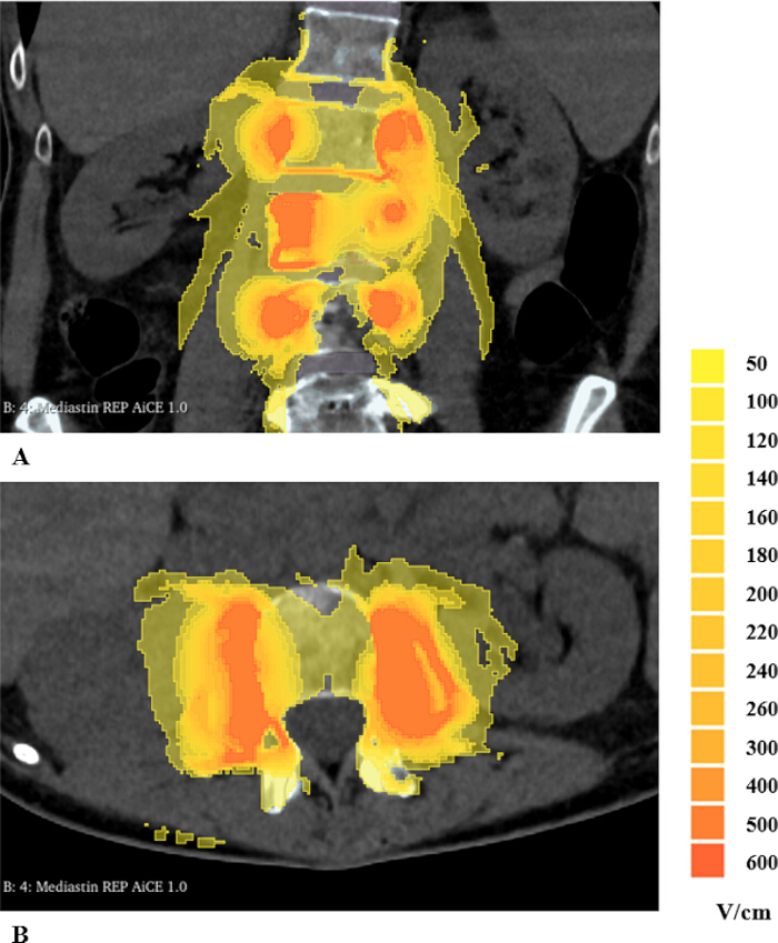
Figure 1: Electric field simulation using the AI4DEEP module in 3D Slicer. Numerical field modeling was performed from procedural inputs (electrode geometry, active length, applied voltage) and tissue conductivities sourced from the IT’IS database. Color-coded isodose maps ranging from 50–600 V/cm are overlaid on intra-procedural CT images in coronal (A) and axial (B) planes, enabling visual assessment of predicted tumor coverage and exposure of adjacent neural structures. Please click here to view a larger version of this figure.

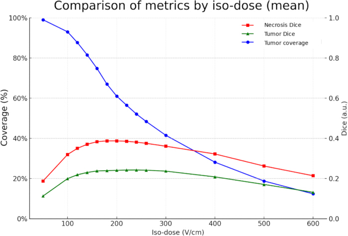
Figure 2: Mean metrics across simulated electric field thresholds. Tumor coverage (blue curve) decreases as the field threshold increases. Dice coefficients follow a bell-shaped distribution, peaking at approximately 160–200 V/cm for necrosis (≈0.38). Please click here to view a larger version of this figure.

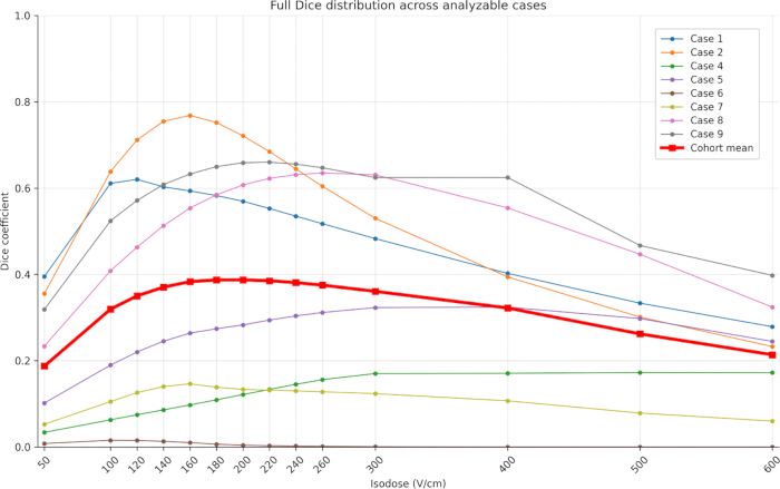
Figure 3: Per-case distribution of Dice similarity coefficients between simulated isodose volumes and post-treatment tumor necrosis. Dice similarity coefficients were calculated on full 3D volumes between segmented post-treatment tumor necrosis and each simulated electric-field isodose volume from 50–600 V/cm. Thin colored lines represent individual cases, and the thick red line represents the cohort mean. Despite substantial inter-case variability, the mean curve showed a bell-shaped distribution, with maximal concordance around 160–200 V/cm. Please click here to view a larger version of this figure.

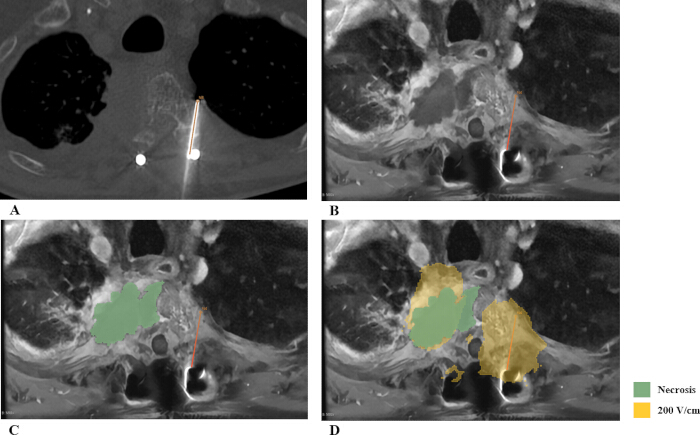
Figure 4: Representative example of post-treatment necrosis segmentation overlaid with the selected simulated isodose volume. (A) Axial intra-procedural CT with electrodes in place (CTa), used to segment electrode position and define treatment geometry. (B) Axial follow-up MRI at best response (MRIs) after rigid registration with initial intra-procedural CT (CTi). (C) Manual segmentation of the post-treatment necrotic area on MRIs (green). (D) Direct 3D overlay of the necrosis segmentation and the selected simulated 200 V/cm isodose volume (yellow). For this patient, Dice similarity at 200 V/cm was 0.28. Please click here to view a larger version of this figure.

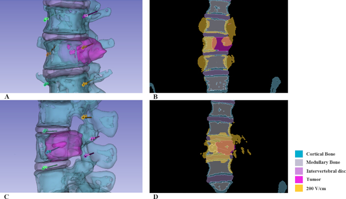
Figure 5: Electric field simulation consistent with anti-tumoral response. A 59-year-old patient with an L3 epiduritis from cholangiocarcinoma underwent an initial procedure that failed (A,B) and was retreated one month later using an alternative needle configuration (C,D), leading to a complete response. (A) Oblique coronal 3D view of needle placement during the first procedure. (B) Electric field map (200 V/cm isodose) showing insufficient tumor coverage. (C) Oblique sagittal 3D view of needle placement during retreatment. (D) Electric field map (200 V/cm isodose) showing tumor coverage exceeding 90%. Please click here to view a larger version of this figure.

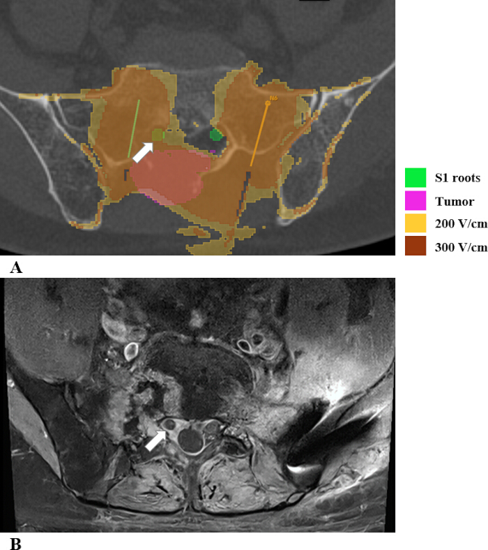
Figure 6: Electric field simulation consistent with observed neural damage. A 67-year-old man with clear cell renal cell carcinoma and L5–S1 epidural disease. (A) Electric field simulation showing the 200 V/cm and 300 V/cm isodoses in yellow and brown, respectively. The right S1 nerve root (arrow) is included within the simulated field, likely because of cortical breach and electrode proximity, whereas the left nerve root is spared. (B) Post-treatment MRI confirming right S1 nerve root involvement (arrow), in agreement with post-procedural right-sided radicular pain and sensory deficit. The left side remained normal on imaging and clinically asymptomatic. Please click here to view a larger version of this figure.

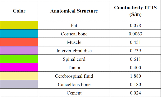
Table 1: Electrical conductivity values used for field simulation. Each anatomical structure was assigned its corresponding IT’IS conductivity value (S/m) and visual color code for segmentation and modeling. Please click here to view a larger version of this table 1.

Case	Best Dice for necrosis	Best isodose (V/cm)	Tumor coverage at best isodose  (%)	Best response (0 = stable disease or progression, 1 = partial response, 2 = complete response)	Adverse event	Adverse event type
1	0.62	120	60	2	0
2	0.77	160	86	1	1	Left L4-L5 radicular pain
3	N/A	N/A	N/A	2	0
4	0.17	500	27	1	0
5	0.32	300	48	1	1	Right C8 radicular pain
6	0.02	100	91	1	0
7	0.15	160	85	2	0
8	0.64	260	83	1	0
9	0.66	220	64	2	1	Right L5-S1 Radicular pain, hypoesthesia and impaired proprioception

Table 2: Per-case quantitative results. The best Dice for necrosis corresponds to the highest Dice similarity coefficient obtained across all tested isodose volumes when compared with post-treatment tumor necrosis. The best isodose corresponds to the isodose associated with the highest Dice value. Tumor coverage at the best isodose, best clinical-radiological response, and procedure-related adverse events are also reported.

Discussion

This protocol provides a reproducible workflow for patient-specific electric field simulation in spinal ECT. Several methodological steps are critical for obtaining accurate and clinically interpretable predictions. Precise tumor segmentation is essential, as epidural disease is often poorly visualized on non-contrast intra-procedural CT. Fusion of pre-procedural and post-procedural MRI is therefore key for accurate delineation of epidural and vertebral involvement. In practice, image fusion may rely on manual rigid registration with visual control and target registration error (TRE) measurement, or on dedicated deformable multimodal registration approaches when more advanced alignment is required, such as patch-based field-of-view matching²⁶. Accurate recording of electrode activation pairs and applied electric field amplitude in V/cm is equally critical, as any mismatch between procedural parameters and the model directly affects simulated field distribution. Careful registration of intra-procedural CT with needles to the planning CT, combined with manual adjustment of active tip electrode segments in multiplanar reconstruction, is also required to ensure that the modeled geometry faithfully reflects the clinical configuration.

Several practical considerations emerged during model implementation. The workflow requires sufficient computing resources, with at least 16 GB and preferably 32 GB of RAM to ensure stable and quick simulations. Metal artifacts on CT can artificially lead to overestimation of segmented coils, cement, or liquid embolic when using threshold-based tools, making manual correction necessary to avoid distortion of conductive structures. Processing very large segmentations, such as full-body fat, lung, or muscle masks, can overload memory, especially when more than ten tissue conductivities are assigned. In these cases, restricting segmentation to the anatomical region of interest improves stability and reduces computation time. These troubleshooting elements are important to maintain reproducibility across workstations and centers.

This method has several limitations. Segmentation is predominantly manual and was performed by a single operator in this study. As a result, the process remains time-consuming, precludes intra-procedural use in its current form, and does not allow evaluation of inter-operator reproducibility. The model relies on linear, static conductivity values and does not account for dynamic conductivity changes occurring during electroporation, which may affect spatial field distribution. The absence of pharmacokinetic modeling of bleomycin represents another source of discrepancy: effective electroporation does not guarantee drug availability, and necrosis may be smaller than the simulated electroporated volume in hypoperfused or previously irradiated tumors. Registration inaccuracies between CT and MRI may also affect tumor–isodose comparisons. Dice coefficients were computed on full 3D volumes and remained modest in absolute terms, which is expected in spinal ECT because electrodes may be deliberately positioned at some distance from the epidural tumor to limit the risk of neural injury. In this setting, the main information lies less in the absolute Dice values than in their distribution across isodose thresholds, which was used to identify the range best matching the observed post-ECT necrotic volume.

Compared with existing numerical studies of spinal electrochemotherapy, which have primarily evaluated theoretical configurations or transpedicular approaches in simplified geometries, this protocol offers a fully patient-specific workflow based on real imaging datasets and clinically delivered electrode configurations^15,16. The identification of the 160–200 V/cm range as the most concordant with post-treatment necrosis is consistent with the relative scaling observed in irreversible electroporation using the same numerical method, where a 400 V/cm isodose correlates accurately with local tumor control^22,23. Although the thresholds differ between techniques, the relative relationship between field strength and effective tissue response appears preserved, supporting the relevance of simulation-based planning. However, this range should be considered specific to the current workflow and interpreted as an empirical threshold rather than as a mechanistic ECT threshold applicable to other models, segmentation strategies, or clinical protocols.

This method has several potential applications. It can support pre-procedural planning by testing alternative electrode geometries and assessing tumor coverage before treatment. With future automation of CT/MRI segmentation, the workflow could be integrated into intra-procedural guidance to refine electrode positioning. Incorporating perfusion-based estimations of bleomycin distribution, for example, through pre-procedural perfusion MRI correlated with local drug uptake, could improve the prediction of the effective electroporated volume. Early post-ECT MRI might also help identify the immediate electroporated zone before secondary tissue remodeling, as reported in irreversible electroporation²⁷. Further prospective and multicentric validation will be needed to refine field thresholds, assess inter-operator reproducibility, and define optimal safety margins. A short learning curve is expected, although segmentation accuracy improves after the first few cases, and corrected segmentations can be reused as templates.

Materials

List of materials used in this article

Name	Company	Catalog Number	Comments
3D Slicer	3D Slicer (open-source)	N/A	Version 5.6.2.
AI4DEEP module (3D Slicer extension)	AI4DEEP	N/A	Electric-field simulation module used within 3D Slicer.
Cliniporator VITAE	IGEA	IG0012A	Pulse generator used for electrochemotherapy
Hybrid angio-CT suite (Alphenix 4D CT + Aquilion ONE)	Canon Medical Systems	TSX-305A	Integrated angiography system (Alphenix) and CT scanner (Aquilion ONE) in a single room; used for intraprocedural CT imaging and procedural guidance.
Straight needle electrodes "VGD"	IGEA	IG0E726	Active length: 20 mm / 30 mm / 40 mm (select according to target size and anatomy).
Workstation	Dell	N/A	Dell workstation, intelVPro ISM, Windows 11 - 16 GB RAM; used for image processing and simulations.