This study proposes a multimodal deep learning framework for video summarization by integrating audio-visual features using pretrained GARNN models. Leveraging GRUs, AlexNet, and an adversarial LSTM classifier, the system enhances keyframe detection, reduces redundancy, and achieves high summarization accuracy with an average F-score of 0.985.
Research Article
GARNN-AE-LSTM: A Multimodal Deep Learning Approach for High-Accuracy Video Summarization
Opens in a new tab
In This Article
Summary
Loading...
$$\rightleftharpoonup{xx}$$
$$\longleftharp{xx}$$,
$$\longrightharp{xx}$$,
Abstract
Loading...
$$\rightleftharpoonup{xx}$$
$$\longleftharp{xx}$$,
$$\longrightharp{xx}$$,
Video summarization focuses on creating concise versions of lengthy videos by preserving essential content. This study reveals a multimodal machine learning strategy that integrates visual and auditory information by using pretrained Gated Recurrent Neural Network architectures referred to as GARNN, combining Gated Recurrent Units (GRUs) and AlexNet, to extract audio, image, and visual features. The keyframe detection is improved by removing redundant frames and applying motion-compensated feature reduction, followed by optional PCA-based dimensionality reduction. An adversarial encoder-based Long Short-Term Memory (AE-LSTM) classifier is employed for temporal modeling by achieving high accuracy in summarization. The results got evaluated by using sensitivity, F-scores, and positive predictive values, and the method attained an average F-score of 0.985. A gated AlexNet is introduced in a multimodal GARNN-AE-LSTM framework, where motion-compensated PCA-based reduction eliminates redundancy, GRUs record temporal progression, and gating fine-tunes spatial feature selection, all of which contribute to a more accurate and efficient video summarization system. The improved F1 score demonstrates the model's effectiveness in generating accuracy in video summaries by creating a meaningful video. This approach highlights the potential of multimodal feature extraction and advanced deep learning techniques for robust video analysis and compression.
Introduction
Loading...
$$\rightleftharpoonup{xx}$$
$$\longleftharp{xx}$$,
$$\longrightharp{xx}$$,
Multimodal Analysis (MMA) systems have emerged, combining several modalities like audio, video, text, and sensor data to provide insights into how students learn1. These technologies can aid in gaining a thorough understanding of student behavior and engagement levels by evaluating multimodal data2. However, there are a number of obstacles and restrictions when it comes to creating efficient MMA systems3. There are a ton of digital videos due to the growth of the Internet and security cameras. It is imperative that these videos be compiled into databases. A video summary can be helpful in this situation. The creation of a useful synopsis of the real video is known as video summarizing, and it helps with activity tracking, anomaly detection, and video retrieval4. Video summary can be accomplished using a variety of strategies. These methods fall into one of two categories5, such as extractive and abstractive video summarization.
Because video summarizing requires a lot of computing, efficient methods are needed. If every frame in a movie is examined for selection, the summary process could be slow and lengthy, and processing resources could be spent on identical or similar frames. Moreover, to expedite the process and ensure that only important features are considered, space reduction ought to be done to any set of features6. Techniques for video summarizing can be categorized into four major areas based on the type of audio-visual signals that are produced and shown to the end user7, or their output. To be more specific, the results of video summarization calculations could include: (i) primary frames8, which are sequentially displayed extracted video frames commonly known as static summaries; (ii) video frames9, which are called dynamic summaries; (iii) visual signals10, which enhance summaries for the end user by adding graphical-based syntax to other cues; and (iv) generated by computers, textual annotations11, that are designed to offer efficient summaries of video information.
Summaries based on keyframes are typically smaller than those based on keyshots. Keyframe refers to an individual representative frame selected from the video. Keyshot denotes a short continuous segment of video frames grouped around keyframes. Summary class refers to the classifier's output labeling frames or segments as informative (to be included in the summary) or non-informative (to be excluded). Nevertheless, this benefit comes at the expense of omitting important details in the process of summarizing. For instance, it can be difficult to get the context of the predecessor frame in a keyframe-based summary. It is also devoid of the original sound. To address these issues, keyshot-based video summarizing techniques are therefore frequently chosen. Keyshot-based video summarizing techniques are utilized to create subsets for either long-form or short-form videos. Short and long-form videos typically have durations of less than and more than 10 min, respectively12. Generating keyshot-assisted subsets for short-form videos is impractical and may not be successful due to their already brief replay length. Furthermore, the playback time of long-form videos, particularly movies or sports videos, might surpass 90 min. For such video categories, keyshot-based summary techniques are more useful and efficient in giving users a brief overview.
The subjective nature of video summary makes it a daunting task. This is due to the fact that each user has distinct tastes, even when it comes to comparable video content. This issue can be precisely resolved with the help of the tailored video summarization approach13. The goal of the algorithm is to provide each user with content that is tailored to their interests. Adapted video summaries with ideal durations for new long-form videos (like sporting events) are not readily available, though. Current methods14,15 require massive computer resources to evaluate customer preference data and video footage in order to provide individualized summaries in real time. Real-time, personalized video summaries can be obtained from centralized dedicated servers. Babu Veesam and Satish16 discussed a thorough taxonomic analysis of all the major video summarizing strategies that demonstrate widely used approaches effectively compressing vast amounts of video data. The review classifies and assesses methodologies in relation to their fundamental approaches, which include multimodal integration strategies, deep learning frameworks, and clustering-based methods. Among the noteworthy methods are the KDAN framework, which uses knowledge distillation for supervised summarization, and the SVS_MCO method, which uses DBSCAN clustering optimized by the Artificial Algae Algorithm. Additionally, the review provides sophisticated models such as the Audio-Visual Recurrent Network and the Query-based Deep African Vulture Learning, which have been found to be highly effective in managing dynamic and multimodal video summarization problems.
The inclusion of a gated AlexNet Recurrent Neural Network (GARNN-AE-LSTM) multimodal framework for video summarization is what makes this study novel. This approach improves the accuracy and efficiency of the video summarization process by reducing redundancy with motion-compensated PCA, capturing temporal dynamics with GRUs, and optimizing spatial feature selection using gating methods. In order to provide the video summarization efficiently with reduced complexity, this paper contributes the following: (i) Multimodal Video Summarization: Proposed a framework for generating concise video summaries by integrating both visual and auditory information using a pretrained GARNN model that combines Gated RNNs and AlexNet. (ii) Gated AlexNet for Feature Refinement: Introduced a novel gated mechanism (Sigmoid gate) into AlexNet's dense layer to filter irrelevant spatial features, thereby enhancing the extraction of high-level visual features. The integration with RNN enables effective temporal modeling of frame-to-frame dependencies. (iii) Redundant Frame Elimination: Developed a motion-compensated variance-based approach to remove identical or similar frames prior to keyframe detection, followed by optional PCA-based dimensionality reduction for efficient feature representation. (iv) Accurate Keyframe Detection: Employed an adversarial encoder-based LSTM classifier for temporal modeling, achieving an average F-score of 0.985, thus demonstrating superior summarization accuracy compared to baseline approaches. (v) Efficiency over Transformer Models: Showcased that the proposed GARNN model is computationally efficient, where AlexNet effectively captures spatial features, RNN models sequential dependencies, and the gating mechanism filters out unimportant frames, outperforming transformer-based alternatives in feature selection and summarization.
Access restricted. Please log in or start a trial to view this content.
Protocol
Loading...
$$\rightleftharpoonup{xx}$$
$$\longleftharp{xx}$$,
$$\longrightharp{xx}$$,
This study proposes a multimodal supervised video summarizing method that falls into the generic video summarization category, commonly referred to as video skimming. This includes techniques that concentrate on finding key segments of a larger video to create a temporally condensed version of it. This study suggests a supervised technique to analyze the video stream in 1 s sections that include audio and visual representations, as shown in Figure 1. These segments are then categorized as either "uninteresting" or "informative". As opposed to synthetic or simulated data, "real data" now refers to the actual video datasets utilized for experiments. Video segments that provide important audio-visual signals necessary for summarization -- such as high motion, voice, or scene transitions -- are referred to as "informative segments." "Uninteresting" parts are defined as repetitious or redundant frames that do not add anything new to the synopsis.
The input videos are segmented into frames, and the multimodal features are extracted from each frame using the proposed GARNN model. The audio and visual features are fused and fed as input into the dimensionality reduction phase, where the redundant frames are removed for further processing. Finally, the proposed AELSTM is applied to the reduced data for video summarization. A supervised binary classifier trained with feature representations from the visual, audio, or mixed modalities, called multi-modalities, is used to achieve this.
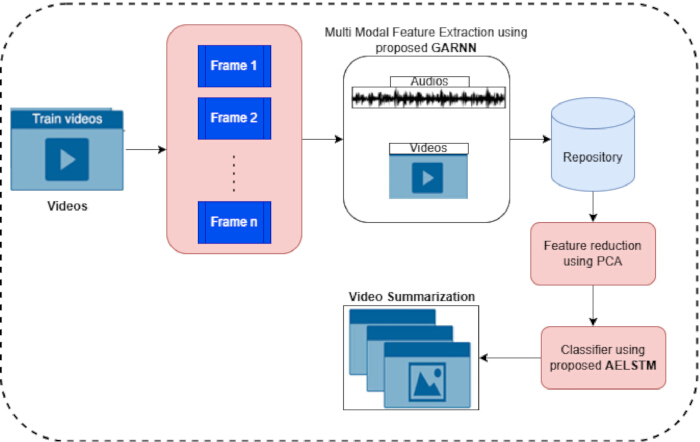
Figure 1: Overview of the proposed video summarization model. The pipeline includes multimodal feature extraction, dimensionality reduction, and summary generation using AELSTM. Please click here to view a larger version of this figure.
Dataset
The effectiveness of the suggested solutions is determined using VSUMM17 and SumMe18 datasets, a pair of benchmark datasets in static video summarization. CNN features created using AlexNet with LSTM and real data are among the datasets. The real data and datasets are accessible to the general public19. The 50 films in the VSUMM dataset are from websites like YouTube and span 110 min at 30 frames per second. They come in a variety of genres, including cartoons, news, sports, advertising, TV series, and home videos. Among these, 25 videos consist of holidays, festivals, and sports that were obtained from the well-known YouTube site and tagged with at least 15 human-generated summaries (390 in total) make up the "SumMe"20 video summary dataset. The duration range of videos is 1-6 min.
The original video is converted into RGB images, which are fed as input into the pretrained proposed GARNN model for feature extraction. This model consists of AlexNet and a gated RNN. The original number of features is 64, and the features from AlexNet have 4100 features.
Proposed Gated-AlexNet-RNN based feature extraction
Both the visual and audio modes of information have been used to summarize the videos. To achieve a feature representation in both modalities, we identified hand-crafted features that are often used in audio and visual clustering and classification tasks, such as picture retrieval, video classification, auditory scene analysis, and music information retrieval. The goal was to include as many instructional visual and audio components as possible. Figure 2 shows a conceptual illustration of the process used to extract features for the audio and visual modalities.
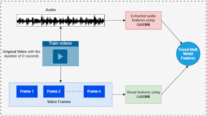
Figure 2: Proposed multimodal GARNN-based feature extraction. Features from both visual and audio modalities are extracted using AlexNet and GARNN components. Please click here to view a larger version of this figure.
Gated- AlexNetRNN: (GARNN)
For virtual image analysis, CNN is a popular DL model21. In general, CNN uses the image as an input and divides it into several groups. Input neurons, a sequence of layers with convolutional pooling, layers that are completely linked, and normalizing layers make up its structure22. The convolution layer's neurons are connected to the preceding layer via a narrow region. The layers underneath them are fully connected to the activating neurons of the fully linked layers. Eqn (1) represents the forward and backward propagation of a fully connected function.
 (1)
(1)
 (2)
(2)
Where  is the activation of ith neuron in lth layer is,
  is the gradient of ith neuron in lth layer,
  is the weight of ith neuron in l+1th layer. Numerous CNN designs have emerged as a result of recent research advancements. AlexNet has been used in this work.
The architecture of AlexNet, shown in Figure 3, reflects a meticulous and well-structured design. Three completely connected layers and five convolution layers make up its eight learning layers. The class labels are produced by feeding the result of the last layer into the function that activates softmax. The second, fourth, or fifth tier kernels are connected to their antecedent levels via GPU sharing. The second and third layer kernels are fully connected to each other. The normalization layer is connected to the max pooling layers after the first and second levels. ReLU is linked to all learning layers.
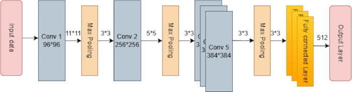
Figure 3: Architecture of AlexNet. Five convolutional layers and three fully connected layers are used to process visual data in the summarization model. Please click here to view a larger version of this figure.
The primary backbone network for the work was a dense-layer GARNN. There are three layers in the thick RNN. With 80 neurons in the second layer and 170 in the first, it is made up of two fully connected (fc) layers. The following layers are batch normalization and dropout. The fc, the last layer, is made up of three neurons and is used to divide up the image. The dense layer, which comes after the LSTM, divides the area around the brain tumor. AlexNet gives the LSTM layer features. The dataset has a maximum of 20 slices, which is equal to the total number of sequences that have been declared. The first layer of the GARNN contains 100 hidden units, whereas the third layer contains 125 hidden units.
The gating mechanism was incorporated into the dense (completely linked) layer of AlexNet in our suggested GARNN-AE-LSTM framework. Convolutional feature maps are often processed by AlexNet and sent straight into fully connected layers for classification. All retrieved spatial characteristics, including redundant or less significant patterns, are treated equally by this method. We addressed this by introducing a gating function that functions as a feature filter and is based on a sigmoid. In mathematical terms, a gate vector g = σ(wX) + b, modulates the dense layer's output, with σ representing the sigmoid function. During training, this gate learns to give various feature activation weights ranging from 0 to 1. They are: (i) low gate values suppress irrelevant features (e.g., background noise or redundant textures). (ii) Higher gate values highlight discriminative features (such as important object regions or motion-sensitive patterns). (iii) This improved feature set is then used by the RNN component, which enables it to better capture temporal dependencies without getting sidetracked by irrelevant spatial information. (iv) Backpropagation is used to change the gating parameters during training in tandem with AlexNet and the RNN. This implies that over time, the model learns which aspects are most important for summarizing in addition to which features to extract.
In Figure 4, the variable X denotes the input data, C denotes the cell, and H denotes the hidden state.
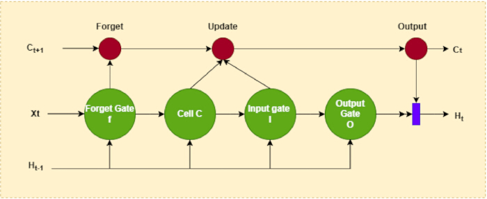
Figure 4: Gated Recurrent Neural Network architecture (GARNN) model. The GARNN integrates batch normalization, dropout, and multiple dense layers for effective sequence modeling. Please click here to view a larger version of this figure.
In each block, the respective weights, such as Iw, Rw, and bias called input, recurrent weight, and bias, respectively, have been utilized as in Eqn (3) to Eqn (5)
 (3)
(3)
 (4)
(4)
 (5)
(5)
At a certain time stamp t, the state of the cell is denoted as in Eqn (6)
 (6)
(6)
Where  the product of Hadamard and the state of hidden unit is denoted as in Eqn (7)
 (7)
(7)
Thus, it utilizes the py Audio Analysis module to compute segment-level audio characteristics for every audio clip that has been extracted from the corresponding video file, utilizing ffmpeg (https: //github.com/tyiannak/pyaudioanalysis)23. The extracted features are listed in Table 1. In accordance with this process, audio feature extraction is initially done on a temporary basis. The final part of the representation is composed of segment-level feature statistics that are calculated at a second level. Specifically, a short-term processing is performed for each segment of the audio signal, resulting in the computation of 68 short-term features (34 features and 34 deltas) for every segment-level window, which may be overlapping or non-overlapping. We have used a variety of visual characteristics to convey the content of the visual information in addition to extracting auditory elements from each video's sound signal. This modality is anticipated to be crucial to the summary process. The multimodal_movie_analysis library (https://github.com/tyiannak/multimodal_movie_analysis) has been used to extract features that reflect visual aspects of a video in order to extract these visual elements. Specifically, the 88 visual elements listed below are taken from the matching frame every 0.2 s. In this, the multimodal features are fused, and a total of 59 features are used for further analysis of classifying the video as informative and not interesting by doing the video summarization.
Feature reduction using PCA
The dimension of the features in this study has been reduced by the application of principal component analysis (PCA). The basic characteristics are transformed into key features in order to boost their prominence and importance. PCA has been widely used by numerous researchers in a variety of domains24. The eigenvalues are used to determine the properties. The highest eigenvalue features are selected, while the lowest eigenvalue features are removed.
Following the removal of superfluous frames, PCA is used in this study as an optional feature reduction step. PCA suppresses noise and redundant information by compressing the high-dimensional feature vectors produced by GARNN into a small subspace. This increases the AE-LSTM's computational efficiency while guaranteeing that keyframe detection is dominated by the most discriminative visual and aural clues. In order to balance scalability and accuracy in video summarization, PCA is utilized as a useful tool. The algorithm (Algorithm 1) is provided as Supplementary File 1.
Any frame that is exactly the same as or strikingly comparable to the preceding frame is considered redundant. It is obvious that changing the framerate can have an impact on the proportion of removed video frames. More specifically, as frame rates increase, the similarity between successive frames increases as well, leading to a higher percentage of frames being removed. Now, the dimensionality-reduced features are used to train the ML model, which is called the adversarial AE-LSTM model.
Training using AELSTM
A neural network called a GAN25 is made up of two rival subnetworks: i) a "generator" network (G) that creates data that resembles an unknown distribution, and ii) a "discriminator" network (D) that distinguishes between the created samples and those from actual observations. The aim is to find a generator that maximizes the likelihood of the discriminator committing a mistake while fitting the actual data distribution.
Assume X is the input and E is the prior input noise, X’= g(E) is the sample generated. Using the minimax optimization, learning is formulated:
 (8)
(8)
Where D is qualified to obtain the correct probability of the classification. The components of our developed training model are shown in Figure 5. The selector LSTM chooses the frames subset from the input video sequence X. The selected frames are converted into fixed-length feature E using the encoder-LSTM, followed by the video reconstruction X' using the decoder-LSTM. The classification of X' into real video or summary class is performed by the discriminator-LSTM. In this study, AE-LSTM is used for video summarization with GAN structure for efficient, diverse, and structured video summaries. The AE can eliminate the unnecessary background changes, and the LSTM can detect the scene transitions rather than treating the frames as images, and the GAN, the generator can summarize the video, and the discriminator ensures the summary is diverse
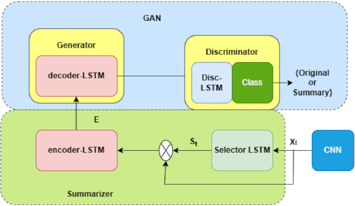
Figure 5: Architecture of the AELSTM summarization model. Includes Selector-LSTM, Encoder-LSTM, Decoder-LSTM, and Discriminator-LSTM to optimize video summaries via adversarial training. Please click here to view a larger version of this figure.
By giving the GARNN features for each frame in the input video X called  , the summarizer utilizes the Selector LSTM to choose the frames subset, and the encoder encodes the frames as E followed by the decoder reconstructing the video as X' at each frame xt. The selector utilizes the importance score when selecting the frame. The features are given by the weight value using the scores, and then move onto the encoder. For each frame with score st = 1, the subset is only received by the encoder. The discriminator chooses the classes as original or summary by estimating the distance between X and X' and assigning the labels. In this case, the discriminator computes the error between the original and summary videos. Algorithm 2 (Supplementary File 2) denotes the summarization of the training of AELSTM for video summarization.
Post-processing – Video summarization
Video summaries can be produced by segment-level classifiers once they have been trained. Three steps are involved in achieving this: (i) Determine each video segment's audio, visual, or blended characteristics. (ii) Classify each video segment using the appropriate audio, visual, or fusion classifier. (iii) To prevent glaring mistakes, post-process the orderly classifier predictions.
To meet this demand, a pipeline consisting of two distinct filters has been developed for the post-processing step. The input array is first subjected to a median filter of length N1 utilizing local windows in order to smooth the sequential classifier predictions. The final predictions are then determined by hard filtering using a straightforward method that maintains a series of consecutively positive predictions (informative segments) if at least N2 segments are included in that sequence. Stated differently, that criterion requires an instructive segment to last at least N2 seconds.
Access restricted. Please log in or start a trial to view this content.
Results
Loading...
$$\rightleftharpoonup{xx}$$
$$\longleftharp{xx}$$,
$$\longrightharp{xx}$$,
The proposed GARNN-based feature extraction and AGLSTM-based video summarization of lengthy videos were experimented on two datasets, namely VSUMM and SumMe. This section discusses the experimental results and comparison with conventional approaches. For the discriminator LSTM, we employ a two-layer LSTM having 1024 hidden units at every layer. For encoder_LSTM and decoder_LSTM, respectively, we employ two two-layer LSTMs having 2048 hidden units in each layer. A decoder LSTM that seeks to store and synthesize the revers...
Access restricted. Please log in or start a trial to view this content.
Discussion
Loading...
$$\rightleftharpoonup{xx}$$
$$\longleftharp{xx}$$,
$$\longrightharp{xx}$$,
In this study, the video summarization of long videos is presented using an efficient multimodal ML and DL models, which use audio, image, and visual modalities of data generated from the input data. The binary classifier is trained to learn the discrimination between the important segments that are the produced summary part and the "non-important" segments that are discarded. The model is trained using datasets such as SumMe and VSUMM, and the scalability of the model is demonstrated in terms of the metrics. Initially, ...
Access restricted. Please log in or start a trial to view this content.
Disclosures
Loading...
$$\rightleftharpoonup{xx}$$
$$\longleftharp{xx}$$,
$$\longrightharp{xx}$$,
The authors have no conflicts of interest.
Acknowledgements
Loading...
$$\rightleftharpoonup{xx}$$
$$\longleftharp{xx}$$,
$$\longrightharp{xx}$$,
The authors are thankful to Dr. Television School, Sichuan Film and Television University, for providing the lab facilities to conduct the research study.
Access restricted. Please log in or start a trial to view this content.
Materials
| Name | Company | Catalog Number | Comments |
|---|---|---|---|
| AlexNet (pre-trained model) | MATLAB / PyTorch | PyTorch Hub — AlexNet pre-trained model: https://pytorch.org/hub/pytorch_vision_alexnet/ | Used for visual feature extraction |
| FFmpeg | FFmpeg.org | https://ffmpeg.org/ | Audio extraction from video |
| GRNN-based model | Custom implementation | Library “neupy” implements GRNN: http://neupy.com/apidocs/neupy.algorithms.rbfn.grnn.html | Used for multimodal feature fusion |
| LSTM (Long Short-Term Memory) | PyTorch | https://pytorch.org/docs/stable/generated/torch.nn.LSTM.html | Used in Selector, Encoder, Decoder |
| Multimodal_movie_analysis lib | GitHub | https://github.com/tyiannak/multimodal_movie_analysis | For visual feature extraction |
| NumPy | Python Software Foundation | https://pypi.org/project/numpy/ | Numerical computation and matrix ops |
| PCA (Principal Component Analysis) | Scikit-learn | https://scikit-learn.org/stable/modules/generated/sklearn.decomposition.PCA.html | Dimensionality reduction |
| PyAudioAnalysis | GitHub | https://github.com/tyiannak/pyaudioanalysis | Audio feature extraction |
| PyTorch | PyTorch Foundation | https://pytorch.org/ | Deep learning framework |
| SumMe Dataset | Public dataset | https://gyglim.github.io/me/vsum/index.html | Benchmark video summarization dataset |
| VSUMM Dataset | Public dataset | http://www.vision.ime.usp.br/~creativision/vsumm/ | Benchmark video summarization dataset |
References
Loading...
$$\rightleftharpoonup{xx}$$
$$\longleftharp{xx}$$,
$$\longrightharp{xx}$$,
- Celik, I., Yildirim, B., Soykan, E. Response of learning analytics to the online education challenges during pandemic: Opportunities and key examples in higher education. Policy Futures Educ. 21 (3), 387-404 (2022).
- Prieto, L. P., Sharma, K., Dillenbourg, P., Muñoz-Cristóbal, J. J., Rodríguez-Triana, M. J. Multimodal teaching analytics: Automated extraction of orchestration graphs from wearable sensor data. J Comput Assist Learn. 34 (2), 193-203 (2018).
- Ouhaichi, H., Spikol, D., Vogel, B. Research trends in multimodal learning analytics: A systematic mapping study. Comput Educ Artif Intell. 4, 100136(2023).
- Basavarajaiah, M., Sharma, P. Survey of compressed domain video summarization techniques. ACM Comput Surv. 52 (1), 129(2020).
- Subba, T., Roy, B., Pradhan, A. A study on video summarization. Int J Adv Res Comput Commun Eng. 5 (1), 14(2016).
- Van der Maaten, L., Postma, E., Van den Herik, J. Dimensionality reduction: A comparative. J Mach Learn Res. 10, 66-71 (2009).
- Money, A. G., Agius, H. Video summarisation: A conceptual framework and survey of the state of the art. J Vis Commun Image Represent. 19 (2), 121-143 (2008).
- Spyrou, E., Tolias, G., Mylonas, P., Avrithis, Y. Concept detection and keyframe extraction using a visual thesaurus. Multimed Tools Appl. 41 (3), 337-373 (2009).
- Li, Y., Merialdo, B., Rouvier, M., Linares, G. Static and dynamic video summaries. Proceedings of the 19th ACM International Conference on Multimedia. , ACM. Scottsdale, AZ. 1573-1576 (2011).
- Sen, D., Raman, B. Video skimming: Taxonomy and comprehensive survey. arXiv. , (2019).
- Video to text SHORT ABSTRACT:SHORT ABSTRACT: Joint video summarization and captioning with recurrent neural networks. Chen, B. C., Chen, Y. Y., Chen, F. Proceedings of the British Machine Vision Conference (BMVC), , BMVA. London, UK. (2017).
- Short form and long form videos. Google Ads Help. , Google. https://support.google.com/google-ads/answer/2382886 (2025).
- Babaguchi, N., Kawai, Y., Ogura, T., Kitahashi, T. Personalized abstraction of broadcasted American football video by highlight selection. IEEE Trans Multimedia. 6 (4), 575-586 (2004).
- Lei, J., Ren, P., Wang, H., Wang, X., Tian, Q. Action parsing-driven video summarization based on reinforcement learning. IEEE Trans Circuits Syst Video Technol. 29 (7), 2126-2137 (2019).
- Thomas, S. S., Gupta, S., Subramanian, V. K. Context driven optimized perceptual video summarization and retrieval. IEEE Trans Circuits Syst Video Technol. 29 (9), 3132-3145 (2019).
- Veesam, S. B., Satish, A. R. An empirical taxonomy of video summarization models from a statistical perspective. IEEE Access. 12, 173850-173866 (2024).
- Unsupervised video summarization with adversarial LSTM networks. Mahasseni, B., Lam, M., Todorovic, S. Proceedings of the IEEE Conference on Computer Vision and Pattern Recognition (CVPR), , IEEE. Honolulu, HI. 2982-2991 (2017).
- Mujtaba, G., Malik, A., Ryu, E. S. LTC-SUM: Lightweight client-driven personalized video summarization framework using 2D CNN. IEEE Access. 10, 103041-103055 (2022).
- DeAvila, S. E. F., Lopes, A. P. B., da Luz, A., de Oliveira, L. P., da Silva Torres, R. VSUMM: A mechanism designed to produce static video summaries and a novel evaluation method. Pattern Recognit Lett. 32 (1), 56-68 (2011).
- Creating summaries from user videos. Gygli, M., Grabner, H., Riemenschneider, H., Van Gool, L. Proceedings of the European Conference on Computer Vision (ECCV), , Springer. Zurich, Switzerland. 505-520 (2014).
- OverFeat: Integrated recognition, localization and detection using convolutional networks. Sermanet, P., Eigen, D., Zhang, X., et al. Proceedings of the International Conference on Learning Representations (ICLR), , ICLR Banff. Canada. (2014).
- Deep residual learning for image recognition. He, K., Zhang, X., Ren, S., Sun, J. Proceedings of the IEEE Conference on Computer Vision and Pattern Recognition (CVPR), , IEEE. Las Vegas Valley, NV. 770-778 (2016).
- Giannakopoulos, T. pyaudioanalysis: An open-source Python library for audio signal analysis. PLoS One. 10 (12), e0144610(2015).
- A PCA-based distributed approach for intrusion detection in wireless sensor networks. Livani, M. A., Abadi, M. A. Proceedings of the International Symposium on Computer Networks and Distributed Systems (CNDS '11), , IEEE. Tehran, Iran. 55-60 (2011).
- Generative adversarial nets. Goodfellow, I., Pouget-Abadie, J., Mirza, M., et al. Advances in Neural Information Processing Systems (NeurIPS), , Curran Associates. 2672-2680 (2014).
- Srivastava, N., Mansimov, E., Salakhutdinov, R. Unsupervised learning of video representations using LSTMs. arXiv. , (2015).
- Nair, M. S., Mohan, J. Static video summarization using multi-CNN with sparse autoencoder and random forest classifier. Signal Image Video Process. 15 (5), 735-742 (2021).
- Issa, O., Shanableh, T. CNN and HEVC video coding features for static video summarization. IEEE Access. 10, 72080-72091 (2022).
- Apostolidis, E., Mezaris, V., Patras, I. AC-SUM-GAN: Connecting actor-critic and generative adversarial networks for unsupervised video summarization. IEEE Trans Circuits Syst Video Technol. 31 (7), 3278-3292 (2021).
Access restricted. Please log in or start a trial to view this content.
Reprints and Permissions
Request permission to reuse the text or figures of this JoVE article
Request Permission