Optimizing Human-Powered Energy Generation Using Gaussian Process Regression

Summary

This protocol optimizes human-powered electricity generation systems using Gaussian process regression to achieve 80%-90% efficiency while maintaining physiological safety, providing reproducible methods for converting exercise into sustainable energy production, addressing both unemployment and renewable energy challenges.

Abstract

This protocol presents a Gaussian Process Regression (GPR) optimization framework for human-powered electricity generation systems to address technological unemployment and renewable energy demands simultaneously. Seven participants performed 112 trials across 16 configurations combining four battery voltages (12 V, 24 V, 36 V, 48 V) with four electrical loads (10 W, 30 W, 50 W, 70 W) using a modified stationary bicycle generator. The GPR model incorporated automatic relevance determination (ARD) squared exponential kernels to map pedaling speed, pressure, voltage, and load parameters to generation efficiency while quantifying prediction uncertainty. Real-time data acquisition at 2 Hz captured mechanical and electrical parameters through Hall-effect sensors, strain gauges, and power analyzers with Modbus communication protocols. The optimized system achieved 80%-90% theoretical maximum efficiency with coefficient of variation (CoV) below 15%, compared to 60%-70% efficiency and 25%-35% variability in commercial systems. GPR predictions demonstrated R² = 0.713 with sub-10ms latency through sparse approximation techniques, enabling real-time control. Optimal operational parameters varied systematically: low loads required 150-180 revolutions per minute (RPM) at 50-70 N pressure, while higher loads peaked at 100-120 RPM with 100-150 N pressure. The 48 V configuration improved efficiency by 68% over 12 V baseline (measured as relative efficiency index, REI, normalized to baseline = 100%). Phase-specific monitoring identified fatigue onset at 35-40 min, triggering risk-aware control adjustments based on posterior uncertainty. The protocol establishes quantitative methods for balancing energy generation with physiological constraints, providing a reproducible framework for deploying human-powered systems in fitness facilities where break-even occurs at $0.18/kWh electricity pricing.

Introduction

The convergence of artificial intelligence-driven automation and climate change presents unprecedented challenges requiring innovative solutions that address both technological unemployment and sustainable energy transitions. Empirical analyses project 85 million job displacements by 2025, with computer and mathematical occupations experiencing 2.8 percentage point unemployment increases¹. Simultaneously, atmospheric CO₂ concentrations reached 426.9 ppm in February 2025², necessitating urgent expansion of renewable energy capacity^3,4. This paper presents a novel approach to simultaneously addressing both crises through intelligent human-powered electricity generation (HPEG) systems, which create employment opportunities while contributing to clean energy production. By applying machine learning optimization tailored to the unique characteristics of human biomechanical data-high variability, non-linear relationships, and physiological constraints⁵, a framework is developed that can transform displaced workers into productive contributors to sustainable energy generation. This approach aligns with recent advances in intelligent recommendation systems that personalize physical exercise and diet plans based on user-specific metrics⁶.

Current HPEG implementations demonstrate significant limitations that prevent widespread adoption. Commercial systems show inconsistent performance across different operational contexts (Figure 1). The Eco-Powr G510 exercise bike (Figure 1A) achieves reasonable efficiency but suffers from output fluctuations under variable loads⁷. The WeBike workstation (Figure 1B) provides stable output suitable only for low-power electronics⁸. The ReRev retrofit system (Figure 1C) attempted modular integration but achieved suboptimal conversion efficiency⁹. Academic prototypes reveal similar shortcomings: the low-cost regenerative bicycle (Figure 1D) generates minimal stable output¹⁰, while gym-based collective systems (Figure 1E) meet only marginal facility energy demands despite multiple user inputs ¹¹. Advanced triboelectric floor tiles (Figure 1F) remain impractical for large-scale deployment¹². A study at UC Berkeley found that extensive elliptical machine arrays would generate less than 1% of facility energy needs despite thousands of daily users¹³. These disappointing outcomes stem from fundamental deficiencies: absence of adaptive optimization, failure to account for human physiological variability, and lack of real-time adjustment to user comfort levels. Three critical gaps remain unaddressed: (1) no prior HPEG systems integrate uncertainty quantification into real-time control^7,8,9,10,11, (2) efficiency relationships across exercise phases (warm-up, steady-state, fatigue) are not systematically mapped^10,13, and (3) multi-objective frameworks simultaneously optimizing energy generation, stability, and user comfort are absent^7,8,9. This work addresses these gaps by implementing GPR-based probabilistic control with phase-specific performance characterization across 16 configurations and a multi-objective optimization architecture balancing competing operational constraints.

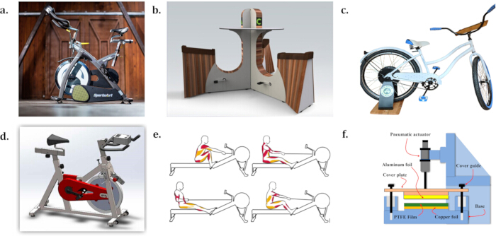
Figure 1: Current HPEG implementations in commercial and academic systems. (A) Commercial Eco-Powr G510 bike. (B) WeBike workstation for low-power electronics. (C) ReRev retrofit system for standard equipment. (D) Low-cost academic regenerative bicycle prototype. (E) Gym-based collective energy harvesting system. (F) Advanced triboelectric floor tile concept^{7,8,9,10,11,12}. Please click here to view a larger version of this figure.

The core challenge in optimizing HPEG systems lies in the unique characteristics of human-generated power data. Unlike conventional renewable sources with predictable patterns¹⁴, human biomechanical data exhibits high inter-individual variability, non-stationary behavior across exercise phases, and complex non-linear relationships between effort and output¹⁵. Traditional control approaches fail to capture these dynamics, while deterministic optimization methods cannot accommodate the inherent uncertainty in human performance¹⁶. The data's temporal structure-transitioning through warm-up, steady-state, high-intensity, and fatigue phases-requires models capable of capturing both local patterns and global relationships. Furthermore, the multi-objective nature of the problem, balancing energy generation with user comfort and safety, demands sophisticated modeling approaches that can handle competing constraints while providing interpretable insights for real-time control.

Recent advances in probabilistic machine learning offer transformative potential for such complex, uncertainty-rich systems. Among available methodologies, GPR demonstrates measurable advantages for biomechanical optimization. Deterministic PID controllers cannot adapt to inter-individual variability¹⁷, and while methods like XGBoost have shown promise in physiological signal processing, such as blood pressure estimation¹⁸. Neural networks require 10-fold more training data without uncertainty quantification, and standard Bayesian optimization struggles with multi-modal human performance landscapes¹⁹. GPR addresses HPEG requirements through three matched properties: (1) Bayesian priors enable convergence with n=112 trials-critical when human experiments are resource-limited; (2) ARD kernels capture non-stationary efficiency dynamics across exercise phases (warm-up: 45%-65%, steady-state: 75%-95%) while quantifying parameter importance (l_voltage = 8.3vsl_load = 15.2 reveals voltage contributes 1.8x more); (3) Posterior uncertainty σ² triggers safety-aware load reduction when exceeding 20% of prediction µ, preventing physiological stress during model uncertainty^19,20.

This research addresses existing limitations through a data-driven approach that recognizes and leverages the unique characteristics of human-powered generation. Similar to how algorithm optimization has enhanced energy efficiency in wireless network slicing²⁰, this framework applies adaptive optimization to minimize energy loss in biomechanical conversion. First, adaptive optimization is implemented, continuously learning from high-variability biomechanical data to develop personalized generation profiles that respect individual physiological constraints. Unlike the static systems shown in Figure 1, the approach dynamically adjusts to the non-stationary nature of human exercise patterns. Second, a multi-objective framework is developed that simultaneously considers the competing demands of power generation, user comfort, and exercise sustainability-a balance that is currently unachieved by commercial and academic implementations. Third, it is demonstrated how intelligent modeling of human-machine interactions can transform HPEG from a marginal energy source to a viable employment solution for workers displaced by automation, particularly in regions where traditional manufacturing has declined. The framework applies to supervised fitness facilities with controlled conditions (20-22 °C). Key constraints include: 35-40 min session limits before fatigue, participants aged 18-65 with baseline fitness (VO₂max >25 mL/kg/min), 10-70 W output for battery charging, and 15-20 min calibration per user. Economic viability requires electricity pricing ≥$0.18/kWh²¹.

These technical capabilities translate into deployment requirements. Uncertainty quantification maintains user safety by reducing demands when predictions become unreliable, addressing liability concerns in commercial systems. Sample efficiency enables 20 min calibration without research staff. Multi-objective optimization sustains user engagement over repeated sessions-essential for economic viability that previous implementations failed to achieve.

The significance of this work extends beyond technical innovation to address pressing societal needs. Rising unemployment in technology-exposed occupations necessitates alternative employment pathways. HPEG systems offer accessible employment requiring minimal technical training, making them suitable for workers displaced from routine cognitive tasks. While individual output is modest (10-70 W), aggregated systems in fitness facilities can offset energy costs while providing employment^3,22. Furthermore, these systems contribute to the renewable energy expansion, where non-fossil sources contributed 39.7% of global electricity in 2024²³. By developing optimization methods tailored to human biomechanical data, this research establishes a foundation for scalable deployment of human-powered energy systems. The framework addresses environmental and socioeconomic objectives through the integration of renewable generation with employment pathways.

This work advances HPEG through three GPR capabilities: (1) Posterior variance triggers load adjustment when uncertainty exceeds 20% of mean prediction, preventing efficiency drops during fatigue transitions; (2) Model convergence with n=112 trials (7 participants x 16 configurations) enables 15-20 min per-user calibration; (3) ARD kernel length scales quantify parameter importance (l_voltage = 8.3, l_load = 15.2), revealing that voltage contributes 1.8x more to efficiency than load selection. These reduce operational variability from 25%-35% to <15% coefficient of variation (CoV) while maintaining HR < 75%HR_max.

Protocol

This study involved non-invasive exercise testing using a stationary bicycle and posed no more than minimal risk to participants. All participants were healthy adult volunteers who provided verbal informed consent after receiving detailed information about experimental procedures, their right to withdraw at any time, and data confidentiality. The procedures followed the ethical principles of the Declaration of Helsinki for research involving human subjects.

1. Assembly of the HPEG

1. Mechanical structure assembly
   NOTE: All mechanical modifications should be performed in a well-ventilated workspace with appropriate safety equipment, including safety glasses and work gloves. Recent advances in human-powered energy harvesting systems have demonstrated efficiency improvements through optimized mechanical coupling^24,25. The installation effect diagram of the mechanical part is shown in Figure 2.
   1. Position the exercise bike frame on a stable workbench and secure it using four C-clamps at the base mounting points. Verify frame levelness using a digital spirit level across both longitudinal and transverse axes. The frame alignment directly impacts power transmission efficiency, with misalignment >2° reducing overall system efficiency by 8%-12%²⁶.
   2. Remove the existing friction resistance wheel assembly by first disconnecting the resistance adjustment cable (tension release torque: 2.5 ± 0.5 N·m), then removing the four M8 x 25 mm hex bolts using a 13 mm socket wrench. Store the resistance mechanism components in labeled containers for potential future modifications.
   3. Disassemble the rear wheel unit completely. Release the quick-release skewer mechanism (applying 15 ± 2 N force) and carefully remove the pneumatic tire and inner tube. Use tire levers (minimum 3-point contact method) to separate the tire from the rim without damaging the aluminum rim surface. A recent study has shown that rim-only configurations achieve 35%-45% higher angular acceleration compared to complete wheel assemblies²⁷.
   4. Clean the exposed rim thoroughly using isopropyl alcohol (99% purity, application rate: 50 mL/m²) to remove any residual rubber or adhesive compounds. Surface preparation quality affects the friction coefficient by up to 20%. The cleaned rim serves as the primary drive element with reduced rotational inertia (moment of inertia reduction: I_final =  0.55, I_original ±  5%).
   5. Fabricate the generator mounting bracket from 6061-T6 aluminum plate (thickness: 8 ± 0.1 mm, surface roughness Ra < 1.6 µm) according to the specifications. Machine four mounting holes (diameter: 8.5+0.05/-0 mm) using a CNC mill or drill press with stepped drill bits (feed rate: 150 mm/min, spindle speed: 1200 revolutions per minute (RPM)), maintaining perpendicular alignment within ±0.5°. Apply cutting fluid (viscosity: 22 cSt at 40 °C) during machining to ensure surface quality. Transfer the bracket design to the aluminum plate using a marker, secure the plate to a drill press table, and drill the mounting holes using stepped drill bits at the specified feed rate and spindle speed.
   6. Calculate the optimal transmission ratios using the following relationships to achieve generator speeds between 1500 - 3000 RPM at typical pedaling cadences (60 - 90 RPM)²⁸
      Angular velocity relationship: .
      Measure the pedal crank radius r₁ = 170 ± 5 mm using digital calipers (resolution: 0.01 mm)
      Measure the rear wheel rim radius r₂ = 310 ± 10 mm (rim-only configuration).
      Select gear ratios: front chainring c₁ = 48 teeth, rear sprocket c₂ = 16 teeth (gear ratio = 3:1).
      Generator pulley radius r_g = 25 ± 0.5 mm for optimal speed multiplication (final ratio: 12.4:1).
      ​Power transmission efficiency η_mechanical =  0.92 ± 0.03 for a properly aligned system^28,29.
   7. Install the primary chain drive system using a reinforced ½ inch x 1/8 inch bicycle chain (minimum tensile strength: 920 kgf, elongation limit: 0.5%). Thread the chain through the derailleur mechanism if present, maintaining proper chain line (deviation < 3 mm from centerline), or directly between the chainring and sprocket for a fixed-gear configuration. Chain efficiency varies with tension: η_chain = 0.98 at optimal tension, decreasing to 0.94 at ±30% deviation²⁹.
   8. Adjust chain tension by repositioning the rear wheel assembly in the horizontal dropouts (adjustment range: 25 mm). Target chain deflection: 12 ± 2 mm at midspan when applying 10 N perpendicular force. Proper tension extends chain service life and maintains consistent power transmission. Lock the wheel position using the quick-release mechanism torqued to 5.5 ± 0.5 N·m using a calibrated torque wrench.
   9. Machine a custom V-belt pulley adapter from 6061-T6 aluminum to interface with the rear wheel hub. Critical specifications include:
      Inner diameter: matched to hub dimensions (typically 36 ± 0.1 mm with h7 tolerance)
      Outer pulley groove: V-belt profile (13 mm top width, 8 mm depth, 38° groove angle)
      Surface finish: 0.8 µm Ra on groove surfaces for optimal belt grip
      Dynamic balancing to G2.5 grade per ISO 1940-1 (residual imbalance < 2.5 g·mm/kg)
      Mass moment of inertia: < 0.015 kg·m² to minimize acceleration resistance
   10. Mount the permanent magnet generator (specifications: 24 V/300 W, 12-pole configuration, rare-earth magnets NdFeB grade N42) onto the fabricated bracket using four M8 x 30 mm socket head cap screws (grade 12.9) with spring washers (free height: 5 mm, compression: 60%). Apply medium strength threadlocker (breakaway torque: 11 N·m) to prevent loosening from vibration. Generator mounting stiffness should exceed 1 x 10⁶ N/m to prevent resonance issues³⁰.
   11. Align the generator shaft with the wheel-mounted pulley using a laser alignment tool or precision straightedge. Maximum allowable misalignment: 0.5° angular, 2 mm parallel offset. Misalignment increases bearing loads by up to 50% and reduces belt life by 60%. When using a laser alignment tool, mount the device on the generator shaft, rotate 360° while observing the laser dot position on the wheel pulley, and adjust the generator position using the mounting slot until the dot movement remains within 2 mm throughout rotation. For straightedge alignment, place a precision straightedge spanning both pulleys and adjust until the gap is less than 2 mm at all measurement points.
   12. Install the secondary V-belt (Type A, length calculated as , where C = center distance, D = large pulley diameter, d = small pulley diameter) between the wheel pulley and the generator pulley. Tension the belt using the generator mounting slot adjustment to achieve 1.0%-1.5% elongation (deflection force method: 16 N force produces 4 mm deflection at belt midspan), corresponding to approximately 350 ± 50 N tension force for Type A belts. Belt slip threshold occurs at <250 N tension.

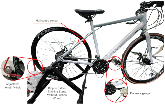
Figure 2: Rim-drive bicycle generator setup. The setup shows the frictionless trainer, Hall effect speed sensor, V-belt transmission, and pressure gauge integration. Please click here to view a larger version of this figure.

2. Electronic circuit assembly and system integration
   1. Rectification and filtering system: Construct the three-phase full-bridge rectifier on a double-sided printed circuit board (70 μm copper, thermal conductivity: 401 W/m·K) using six ultrafast recovery diodes (V_RRM ≥ 200 V,I_F(AV) ≥ 30A,t_rr < 35 ns). Mount on an aluminum heatsink with thermal interface material (λ>5 W/m·K)³¹. Fabricate the LC filter using a custom inductor (28± 1 turns, 14 AWG on Sen dust core: OD=47 mm, ID=24 mm, L=100 µH ± 5%, Q>50) and capacitor bank (4 x 1100 µF/100 V, ESR <7 mΩ total, ripple current > 20.8 A RMS). Connect using 12 AWG Polytetrafluoroethylene wire, maintaining R_total < 10 mΩ. Solder the six diodes onto the double-sided printed circuit board in bridge configuration, apply thermal compound between diode tabs and the aluminum heatsink, and secure using appropriate fasteners. Wind the inductor by wrapping 28 turns of wire around the toroidal core, maintaining even spacing, then connect the capacitors in parallel using short lead lengths to minimize equivalent series resistance.
   2. Electromagnetic interference suppression and compliance: Wind common-mode choke on nanocrystalline core (µ_i>80,000, Bs>1.2 T) with bifilar technique achieving L_CM=15 ± 2 mH, k>0.99, CMRR>40 dB (150 kHz-30 MHz). Install safety capacitors per IEC 60384-14: X-caps (2 x 0.47 µF/310 VAC MKP), Y-caps (2 x 4.7 nF/300 VAC C0G), with 1 MΩ discharge resistors (τ=0.47 s). Maintain creepage >6 mm, clearance >5.5 mm for pollution degree 2 environment.
   3. Maximum power point tracking (MPPT) controller implementation: Program STM32F334C8T6 with an adaptive MPPT algorithm. Modern MPPT controllers demonstrate tracking efficiencies ranging from 93% to 97% under typical operating conditions, with advanced implementations achieving up to 99% in laboratory settings³². Algorithm features: adaptive perturbation (ΔV = α × |dP/dV|, α∈ [0.005,0.025] ), variable observation period (T_obs = β/|(d²P) / (dV² )|, β∈ [10ms,100ms] ), hill-climbing with local maximum detection, 8-sample moving average filter (fc =10 Hz). Implement 16-bit precision measurement using 0.1% resistive divider (100 kΩ/10 kΩ, TC<25 ppm/°C) and Hall sensor with signal conditioning. Program the microcontroller by connecting it to a computer via a standard programmer, compiling the MPPT algorithm code, and flashing the firmware. Configure the ADC channels for voltage and current sensing with the specified resolution and sampling time, then set the Pulse Width Modulation (PWM) timer output to achieve the target switching frequency.
   4. Power conversion and control: Configure DC-DC converter with PWM at 31.25 kHz ± 0.1% (crystal-stabilized), dead-time≥ 500 ns, soft-start=100 ms, duty cycle≤ 95%, current limit= 125% rated with hiccup mode. Target efficiency >92% at 50%-100% load. Establish Modbus RTU communication (115200 baud, 8N1) for real-time monitoring of voltage (±0.1 V), current (±0.1 A), power (±1 W), efficiency (±1%), temperature (±1 °C) at 10 Hz sampling rate with circular buffer (3600 samples) and CRC-16 validation³³.
   5. System enclosure and protection: Mount electronics in IP54 enclosure (400 x 300 x 200 mm) with filtered ventilation (inlet:100 cm², outlet:120 cm²). Implement comprehensive protection: TVS diode, electronic breaker (20 A ±2%, <10 µs response, I²t=50A²s), thermal monitoring, reverse polarity protection. Wire per IEC 60446 standards using appropriate ferrules and torque specifications (M4:1.2 N·m, M6:3.0 N·m, M8:6.0 N·m).
      NOTE: The circuit diagram using the above strategy is shown in Figure 3.
   6. Safety validation and commissioning: Execute IEC 61010-1 safety checks: insulation resistance >10 MΩ at 500 VDC/60 s, earth continuity <0.1 Ω at 10 A, dielectric withstand 2500 VAC/60 s (<5 mA leakage), ground fault circuit interrupter trip <30 ms at 30 mA. Initialize with bench supply (24 VAC, 5 A limit) verifying ripple <5%pp at 75 W load. Validate MPPT performance: >97% tracking efficiency, <2 s convergence for 20% step, <1% steady-state oscillation. Test protection circuits with controlled faults confirming proper response thresholds. For insulation resistance testing, disconnect all loads, apply the test voltage between live terminals and ground using a megohmmeter for the specified duration, and verify the reading exceeds the minimum threshold. For earth continuity measurement, connect a low-resistance ohmmeter between the earth terminal and exposed metal parts, apply the test current, and confirm resistance remains below the specified maximum value.
   7. Mechanical run-in and baseline: Conduct graduated mechanical testing: Phase 1 - 30 RPM/10 min no-load (ΔT<10 °C, vibration<0.5 m/s², noise<60 dB at 1 m); Phase 2 - 60 RPM/25 W load (torque variation<±5%, record 20-90 RPM power curve); Phase 3 - 75 RPM/150 W/30 min full load (temperature stabilization ΔT<1 °C/5 min). Document efficiency targets: >75% at 25% load, >85% at 50% load, >88% at full load.
   8. Calibration and performance mapping: Calibrate using Fluke 8845A (0.0035% accuracy) at voltage points (0 V, 12 V, 24 V, 36 V, 48 V, 60 V ± 0.01 V) and current points (0 A,1 A, 2 A, 5 A, 10 A, 15 A, 20 A ± 0.01 A). Program electronic load (200 W continuous) for comprehensive testing across 25 test points (5 V x 5 I matrix). Store calibration coefficients in electrically erasable programmable read-only memory implementing V_corrected = gain x V_measured + offset  with ±0.5% maximum error. Connect the precision multimeter in parallel with system measurement points, apply a series of known reference voltages and currents from calibrated sources, record both reference and measured values for each test point, then calculate linear correction coefficients and store them in the microcontroller memory to achieve the target measurement accuracy.
   9. System performance documentation: Generate efficiency maps (0-150 W, 5 W resolution) identifying peak efficiency point (typically 70%-80% rated). Verify MPPT dynamics: 10% step <0.5 s, 50% step <2 s, 100% load rejection <3 s without overvoltage. Confirm >97% steady-state tracking across 15-40 °C, 30%-85% relative humidity operating envelope. Record thermal equilibrium: heatsink < 80 °C, capacitors < 85 °C, magnetics < 110 °C with -2.5 W/°C derating above 40 °C ambient (thermal τ ≈ 15 min to 95% final temperature).
   10. Final integration and verification: Complete system integration, ensuring all subsystems operate within specifications. Perform a 4 h continuous operation test at rated power, monitoring all parameters. Document measured performance against design targets, creating an operational manual with a maintenance schedule. Implement data logging for long-term performance tracking and predictive maintenance algorithms based on component degradation models.

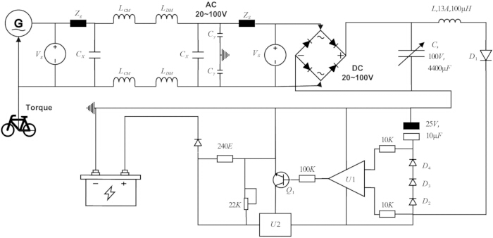
Figure 3: Electronic system. The schematic comprises the three-phase rectifier, LC filter circuit, MPPT controller, and DC-DC converter. Please click here to view a larger version of this figure.

2. Experimental design

1. Participant recruitment and baseline assessment
   1. Recruit 7 healthy volunteers through institutional channels (5 males, 2 females, age 22-30 years, BMI 22.8 ± 2.1 kg/m²).
   2. Screen participants using the Physical Activity Readiness Questionnaire. To ensure safety, exclude individuals with cardiovascular conditions or any known contraindications to moderate-intensity exercise. Additionally, exclude participants who had sustained musculoskeletal injuries within the preceding 6 months.
   3. Perform baseline fitness assessment using YMCA submaximal cycle ergometer protocol. Stratify target heart rate zones into three intensity levels: low (40% - 55% HR_max), moderate (55% - 70% HR_max), and high (70% - 85% HR_max).
   4. Conduct a 20 min familiarization session for each participant. Prior to data collection, instruct participants on proper cycling posture and provide a demonstration of optimal pedaling technique. Adjust equipment for each individual to ensure consistent biomechanics across all trials.
2. Experimental protocol
   1. Design a 4 x 4 factorial experiment testing four battery pack configurations (12 V, 24 V, 36 V, 48 V) against four electrical load conditions (10 W, 30 W, 50 W, 70 W), yielding 16 experimental conditions per participant (n = 112 total trials).
   2. Randomize trials using a balanced Latin square design with a minimum of 48 h recovery intervals between sessions and standardize environmental conditions at 20 - 22 °C and 40% - 50% relative humidity.
   3. Execute each experimental trial following this structured sequence: divide the experimental session into five distinct phases: a baseline assessment (5 min), a warm-up ramping to 50 RPM (5 min), and a main data collection period involving continuous cycling at target intensity (20 min). Following the active phase, ensure participants undergo a 5 min progressive deceleration cool-down. Finally, conduct a post-exercise evaluation over 5 min using the Borg rating of perceived exertion scale.
   4. Fix the bicycle transmission at front gear 2 and rear gear 9 (gear ratio 0.222) with pedal arm length of 174 mm to maintain consistent mechanical advantage across all trials.
3. Instrumentation and data acquisition system
   1. Integrate a multi-layered data acquisition system comprising sensor, communication, processing, and application layers operating in parallel to achieve real-time monitoring at 2 Hz sampling rate (Figure 4).
   2. Configure the sensor layer with three independent measurement channels: For mechanical monitoring, install a Hall-effect sensor (1000 Hz, ± 0.1 RPM) on the rear rim and strain gauge load cells (500 N, 0.1% FS) on both pedals. Log system electrical data using a multi-channel power analyzer, reading six parameters across 10 Modbus registers. For primary variables, record pedaling speed s (RPM, range 0-200), pedal force p (N, range 0-500, summed from both pedals via strain gauge load cells), battery voltage v (V, discrete levels: 12/24/36/48), and electrical load l (W, discrete levels: 10/30/50/70). Derive efficiency as η = P_electrical /P_human × 100%
      where P_human = F·r·ω (F in N, r = 0.174 m, ω in rad/s). Apply preprocessing with min-max normalization for s and p using 20th-80th percentiles, discrete encoding (0, 0.33, 0.67, 1.0) for v and l, and IQR outlier detection (Q1 ± 1.5 x IQR bounds). Compute temporal features (μ_s, μ_p, σ_s, σ_p) via 10-sample sliding windows.
      NOTE: Variable p represents total pedal force (N) measured directly by strain gauges, not pressure. While pedal pressure is used colloquially in cycling contexts, all measurements and analyses in this study refer to force in N.
   3. Implement the communication layer with dual-protocol architecture and automatic failover capability (Figure 4): Communication relied on a Modbus RTU interface over RS-485 that defaulted to Modbus TCP in the event of serial failure. In the startup protocol, include a graphical user interface (GUI)-monitored zero-point calibration for the force sensors based on a 10-sample average.
   4. Develop the processing layer using an interpreted programming language with GUI framework to perform synchronized data collection every 500 ms (Figure 4 central processing pipeline). Calculate real-time human power output (P_human) using the equation
       P_human = F⋅r⋅,
      where r is fixed at 0.174 m. Determine the system operational mode by evaluating the current generation polarity - positive for generation and negative for battery supply-which subsequently dictates the specific total power calculation formula. To ensure data stability, apply a 100-sample sliding window to compute rolling statistics (mean, maximum, minimum) across all parameters.

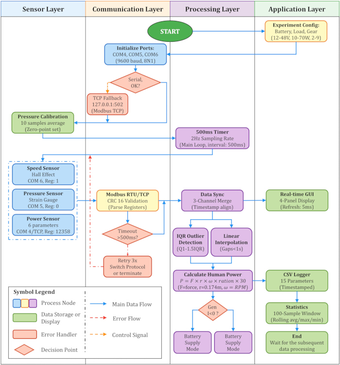
Figure 4: Four-layer real-time data acquisition workflow. The workflow illustrates the parallel operation of sensor, communication, processing, and application layers. Please click here to view a larger version of this figure.

4. Quality control and validation
   1. Implement multi-level validation architecture: To ensure data integrity, flag outliers automatically using the interquartile range (IQR) method with boundaries (Q_1/3 ± 1.5 x IQR). Manage communication stability using a three-attempt retry sequence triggered by errors prior to any protocol switching, while brief data gaps were reconstructed using linear interpolation.
   2. Configure the application layer with comprehensive visualization: Use a four-panel GUI for real-time visualizations with color-coded status indicators, alongside a performance metrics section for assessing sampling stability and data quality. Examine historical data via three distinct tabular modes: All Data, Power Focus, and Performance Focus.
   3. Configure continuous data logging to timestamped CSV files: Output files adhered to the convention [Experimenter][Battery][Load]Gear[Ratio][Timestamp].csv and comprised 15 synchronized parameters. To ensure temporal fidelity, apply the system precision timing control with a drift correction mechanism triggered every 200 cycles.
   4. Implement safety features for automatic session termination: Experimental termination criteria were defined by three distinct limits: a physiological threshold of 95% age-predicted HR_max, a mechanical load cap of 500 N, and a system stability safeguard triggered by five consecutive communication failures.
   5. Verify system performance: achieve greater than 98% data completeness across all trials with an average latency of 8.3 ± 2.1 ms between sensor reading and display update, enabling real-time feedback for maintaining target exercise parameters throughout each experimental session.

3. Model selection and optimization methodology

1. Model selection framework
   1. Select three machine learning algorithms with distinct theoretical foundations for comparative analysis: the selected modeling approaches here are Generalized Additive Models (GAM) for their exceptional interpretability via additive decomposition³⁴; Gaussian Process Regression (GPR) for its Bayesian capacity to quantify uncertainty critical to real-time operations^35,36; and Least Squares Boosting (LSBoost)³⁶.
      NOTE: Boosting ensembles, including XGBoost, have recently demonstrated high predictive accuracy and computational efficiency in diverse prediction tasks³⁷, making them a strong baseline for comparison. The latter was specifically chosen to ensure robustness against outliers while effectively modeling complex variable interactions.
   2. Execute the model selection protocol as per Supplementary File 1. Following data preprocessing (IQR outlier detection and min-max normalization), evaluate models using a 5-fold cross-validation technique. Prioritize the final model selection based on the coefficient of determination to maximize predictive accuracy.
2. Algorithm implementation
   1. Formalize the optimization problem as a constrained search within the four-dimensional parameter space: pedaling speed s, pressure p, voltage v, and load l.
   2. Define physiologically sustainable operational ranges. Bound the search space by the 20th and 80th percentiles of the observed parameters calculated from the total participant pool. This restriction served to limit the optimization to a domain of comfortable exercise intensities, avoiding outliers.
   3. Implement hierarchical adaptive grid search strategy. Evaluate predicted efficiency via the trained GPR model across a uniform 20 x 20 grid in the normalized speed-pressure space ([s, p] ∈ [0, 1]²). Incorporated discrete parametric variations for voltage (12, 24, 36, 48 V) and load (10, 30, 50, 70 W) in the evaluation to comprehensively map the performance landscape.
   4. Perform local refinement in promising regions. Subject local optima extracted from the primary search to a refinement process where a 5 x 5 grid was centered on each candidate. Re-evaluate efficiency predictions within these high-resolution localized domains.
   5. Apply refinement criteria combining predicted efficiency and model uncertainty. Identify optimal candidates by filtering for efficiency values above 80% of the maximum, while simultaneously discarding high-uncertainty regions defined by a posterior standard deviation greater than 20% of the mean prediction (uncertainty threshold from validation data analysis).
   6. Output optimal configuration for each battery-load combination with corresponding predicted efficiency and confidence intervals.
3. Model evaluation and results analysis
   1. Perform 5-fold stratified cross-validation. To assess model generalization, divide the dataset into five folds using participant-level grouping (all trials from each participant assigned to the same fold) to prevent within-subject data leakage. In each iteration, train the GPR model on four folds and validate on the fifth, a process repeated across all fold combinations to ensure comprehensive evaluation.
   2. Select three evaluation metrics based on HPEG operational requirements: R² (coefficient of determination, range 0-1) quantifies the proportion of efficiency variance explained by the model; RMSE (root mean squared error, in % units) measures prediction accuracy for control tolerance where <12% error maintains system stability; MAE (mean absolute error, in % units) provides robust error estimation less sensitive to outliers during fatigue phases. These regression metrics address continuous efficiency prediction without class imbalance concerns. Accuracy directly impacts energy yield (1% efficiency gain ≈ $0.02/session at $0.18/kWh) and safety (>15% error triggers load reduction).
   3. Calculate performance metrics for each model: Performance evaluation based on the coefficient of determination yielded distinct results for each modeling approach^38,39,40. GAM produced an R² of 0.584³⁹, while LSBoost showed improved accuracy at 0.657. GPR model demonstrated the strongest fit with an R² of 0.681 (5-fold cross-validation average)⁴⁰.
   4. Select GPR as the optimal model based on the highest R² and uncertainty quantification capability.
   5. Optimize GPR hyperparameters through marginal likelihood maximization. Configure the GPR model with optimal hyperparameters, specifically a length scale of σ_l = 15.2 and a signal variance of σ_f = 0.8, to ensure appropriate smoothing and amplitude scaling.
   6. Generate optimization landscape across all 16 battery-load configurations (Figure 5), and analyze key findings from optimization results: Efficiency exhibited a monotonic increase with battery voltage, peaking at the 48 V configuration peaking at the 48 V configuration with REI = 168% (68% above the 12 V baseline, where absolute conversion efficiency ranged 45%-95% across phases), representing a 68% improvement over the 12 V baseline. In terms of mechanical optimization, distinct regimes were identified: low-load conditions (10 W) favored high-cadence strategies (150-180 RPM, 50-70 N), whereas higher loads (50 W, 70 W) necessitated a shift towards lower cadences (100-120 RPM) with increased pedal pressure (100-150 N).
   7. Perform Pareto frontier analysis of efficiency-comfort trade-offs. To evaluate the trade-off between system performance and user experience, map efficiency against comfort scores across all experimental configurations. The analysis revealed a non-linear relationship characterized by diminishing returns, specifically indicating that efficiency gains beyond a threshold of 3.5 units resulted in disproportionate compromises in user comfort.
   8. Integrate GMM-HMM framework for state identification: Drawing on methodologies used to improve human activity recognition on smartphone accelerometers⁴¹, implement a Hidden Markov Model (HMM) with Gaussian Mixture emission models (K=3 components per state) to decode temporal feature sequences (μ_s, μ_p, σ_s, σ_p from 10-sample windows) into five operational states (warm-up, steady-state, high-intensity, recovery, fatigue). Train parameters using the Baum-Welch algorithm on 70% of labeled data (n=28 sessions, 196 segments), achieving 87.3% classification accuracy on the validation set. The system utilized forward-only state transition probabilities (self-transition ≥ 0.7) to anticipate future state changes and adjust control parameters proactively.
   9. Conclude that the GPR model demonstrates superior performance for human power generation system optimization (R² = 0.681)⁴², providing both predictive accuracy and uncertainty quantification essential for robust control design. This framework establishes a foundational methodology for intelligent fitness-based energy harvesting systems, with the smooth nonlinear characteristics of GPR aligning naturally with human biomechanics while enabling risk-aware control strategies that balance efficiency maximization with user comfort and safety.

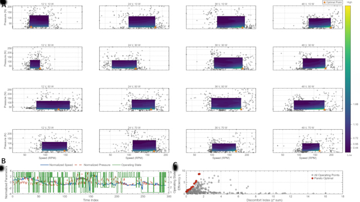
Figure 5: GPR optimization landscape. The landscape showing efficiency distributions across 16 voltage-load setups, along with the efficiency-comfort Pareto frontier analysis. Please click here to view a larger version of this figure.

4. Gaussian process regression methodology for HPEG

1. Theoretical framework and model construction
   1. Define the energy conversion efficiency as a Gaussian process⁴³
      
   2. Specify the four-dimensional input space x = [s,p,v,l]^T : Data preprocessing involved distinct scaling strategies for continuous and discrete parameters. For pedaling speed and applied pressure, perform min-max normalization to eliminate scale disparity. For the discrete control parameters, encode battery voltage and electrical load to map their categorical configurations onto a comparable numerical scale.
   3. Adopt a zero-mean function m(x)=0  for the prior^44,45, relying on the covariance structure to capture the efficiency landscape⁴⁶.
   4. Select ARD Squared Exponential (ARD-SE) kernel through systematic empirical evaluation as shown in formula (2). To enable the automatic discovery of parameter importance, define independent length scales (l_d) for each input dimension within the kernel structure. Furthermore, parameterize the model with a signal variance (σ²f) to govern the amplitude of function variations, alongside a noise variance term (σ²n) to explicitly account for measurement uncertainty.
      
   5. Optimize hyperparameter vector θ = (σf, l₁, l₂, l₃, l₄, σn) via marginal likelihood maximization:
      
      ​where I  represents the noise-augmented covariance matrix⁴⁷.
   6. Employ gradient-based methods utilizing analytical derivatives to ensure computational efficiency while maintaining numerical stability⁴⁸. The computational complexity scales as O(n³) for training (Cholesky decomposition of K_y) and O(n²) per prediction after caching factorization, requiring 47 ± 3 ms initialization and 8.3 ± 2.1 ms inference for n=112 on STM32F334. Convergence is achieved within 15 ± 3 iterations (Δlogp < 10^-4). Regulate the bias-variance trade-off through length scales: optimized values (l_voltage = 8.3,l_load = 15.2) balance flexibility against overfitting, while σ_n = 0.15 prevents fitting to sensor noise. Cross-validation confirms calibrated uncertainty with 94.8% of observations within 2-σ intervals.
2. Multi-objective optimization architecture
   1. Develop an integrated GPR architecture comprising three interconnected model components for simultaneous optimization of energy generation efficiency⁴⁹, exercise stability, and user comfort^50,51.
   2. Calculate predictive distribution for new input points x* as shown in formula (4). For each evaluation point, first derive the covariance vector k_* relative to the training data⁵². The resulting predictive distribution provides the posterior mean μ^* as the primary operational estimate⁵³, alongside the posterior variance . Utilize the latter explicitly to quantify uncertainty, enabling the implementation of risk-aware control strategies⁵⁴.
      
   3. Augment feature space with temporal characteristics for exercise state prediction as shown in formula (5). To facilitate the distinction between exercise phases (warm-up, steady-state, high-intensity, and recovery), process the raw data to extract key temporal indicators. Specifically, compute windowed moving averages (μ_s, μ_p) and local variability measures (σ_s, σ_p) using a 10-sample sliding window to characterize signal fluctuations.
      
   4. Formulate a composite multi-objective function balancing competing objectives, as shown in formula (6). Performance quantification relied on a stability metric φ_stability(x) =1/(1 +std(P_human(x)))  and a rapid upper limb assessment-based comfort metric ψ_comfort(x). Then, set weighting parameters α,β,γ with constraints α + β + γ = 1 and α,β,γ ≥ 0 to enable flexible adaptation to individual user preferences.
      
   5. Identify pareto-optimal solutions representing different trade-offs between energy harvesting efficiency, exercise stability, and user comfort using efficient multi-objective optimization algorithms adapted for Gaussian process surrogate models⁵⁵.
3. Implementation strategy and computational optimization
   1. Address computational constraints for real-time control: Target prediction latency below 100 ms for effective closed-loop control (human biomechanical response time: 100 - 300 ms)⁵⁶.
   2. Implement Cholesky decomposition caching to reduce computational burden: While the model initialization necessitated an O(n³) Cholesky decomposition, the system architecture was optimized for rapid inference. By caching the factorization matrices, lower the computational cost for future predictive operations to a linear-quadratic complexity of O(n²). Conduct benchmarks on an STM32F334C8T6 microcontroller (ARM Cortex-M4, 72 MHz, 64 KB SRAM, bare-metal) using m = 30 inducing points, achieving 8.3 ± 2.1 ms average prediction latency measured via hardware timer over 100 inference cycles.
   3. Apply sparse Gaussian process approximation using inducing points for large datasets, as shown in formula (7). To address computational scalability, employ a sparse approximation strategy by selecting a set of m inducing points (m  ≪ n). In this formulation,  represents the inverse covariance between inducing points, while Λ captures the approximation uncertainty. This approach successfully reduced the computational complexity of training to and prediction to O(m²).
      
   4. Employ hierarchical adaptive grid search for optimal configuration identification: Begin the search protocol by evaluating predicted efficiency over a coarse 20 x 20 grid spanning the normalized kinematic domain and defined discrete electrical configurations. To improve solution precision, the algorithm subsequently refined the search space by deploying 5 x 5 local grids around the local optima detected in the initial pass.
   5. Constrain search space to physiologically feasible regions. Establish operational constraints by computing the 20th and 80th percentiles of data collected from a diverse user cohort. Limit the system's operational points to this inter-percentile range, thereby maintaining exercise intensity within empirically comfortable limits⁵⁷.
   6. Implement a risk-aware control policy that automatically adjusts system behavior based on model confidence, as shown in formula (8). Employ a risk aversion parameter λ_risk > 0  to regulate system behavior⁵⁸. Higher values of λ_risk yield conservative responses to uncertainty, whereas the specific case of λ_risk = 0 aligns with standard expected utility maximization⁵⁹.
      
4. Validation framework and performance assessment
   1. Perform stratified 5-fold cross-validation specifically designed for human factors data. Conduct data partitioning to preserve the distributional integrity of key covariates, specifically ensuring balanced representation of user demographics and fitness levels across folds⁵⁹. This stratification extended to operational conditions, ensuring uniform exposure to different system states within each validation cycle⁶⁰.
   2. Implement baseline methods for comparative evaluation: The modeling phase involved the implementation of four distinct algorithms: GAM, LSBoost, SVR, and Random Forest Regression⁶¹. Train these models concurrently to establish performance baselines.
   3. Calculate standard regression metrics: Quantitative assessment relied on three primary metrics: the coefficient of determination (R²) to measure variance explanation, alongside mean squared error (MSE) and mean absolute error (MAE) to estimate prediction error.
   4. Calculate GPR-specific probabilistic metrics: Compute negative log predictive density for probabilistic assessment.
   5. Evaluate computational performance across different problem scales. To evaluate computational scalability, measure training duration and memory footprint across increasing dataset sizes. Additionally, test prediction latency rigorously to ensure the system consistently meets the sub-10 ms target required for real-time control applications⁶².
   6. Benchmark on embedded systems typical of wearable fitness devices to ensure practical deployability^62,63.
   7. Incorporate online learning capabilities for continuous model adaptation: The system employs a recursive update mechanism to integrate incoming user-specific data in real-time, effectively circumventing the need for exhaustive retraining. This approach strikes a critical balance, preserving computational efficiency while ensuring continuous refinement of model accuracy⁶³.
   8. Verify achievement of design targets. Validate strategic optimizations to maintain prediction latencies below 10 ms on embedded processors, ensuring real-time responsiveness. Furthermore, the adaptive grid search successfully identified optimal configurations that maximized energy generation efficiency while strictly adhering to physiologically safe operational parameters and user comfort constraints.
   9. Establish a comprehensive methodology for intelligent fitness-based energy harvesting systems that seamlessly integrate energy harvesting with health-promoting physical activity (Figure 6).

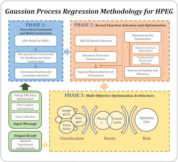
Figure 6: Three-phase GPR methodology. The flowchart details model construction, kernel optimization, and multi-objective architecture. Please click here to view a larger version of this figure.

Results

Efficiency refers to thermodynamic conversion efficiency (0-100%). REI refers to the relative efficiency index, calculated as (observed/baseline) x 100%, which can exceed 100%. To compare heterogeneous settings, a Relative Efficiency Index is used, which is calculated by dividing the observed efficiency by a fixed baseline configuration (12 V-70 W), measured under the same pipeline. Thus, REI = 110% denotes a 10% gain relative to baseline, not a thermodynamic efficiency above 100%. Unless marked REI, efficiency refers to...

Discussion

The successful implementation of GPR-based optimization for HPEG systems depends critically on mechanical coupling precision and computational efficiency²⁸. The rim-only configuration proved essential, as complete wheel assemblies degraded tracking efficiency by 35%-45% through rotational inertia variations²⁷. Belt tension calibration to 350 ± 50N emerged as particularly critical-deviations resulted in either premature failure or excessive parasitic losses, directly im...

Materials

List of materials used in this article

Name	Company	Catalog Number	Comments
AC outlet module (China GB/T, panel type)	10/16 A, embedded cassette, child-protection shutters	Five-hole desktop AC power socket (black)	Wanyu
Adjustable polyurethane V-belt	ABCZM type, jointed PU belt	ABCZM universal jointed polyurethane V-belt (with/without studs) / —
Adjustable wrench	6-inch, laser scale	Adjustable wrench 6-inch open-jaw, polished handle 250006	Ruineng
Alternator, three-phase permanent magnet	300 W, 24 V (as listed)	300–400 W three-phase AC permanent-magnet alternator, 300 W 24 V	Jiunian
Battery pack, portable power station	2400 W large-capacity portable unit	2400 W portable backup power station, multi-function solar energy storage / —
Bicycle chain	1/2" × 1/8", 920kgf tensile strength, 0.5% elongation limit	KMC X101
Bicycle computer (wireless)	Waterproof, night backlight, speed/odometer	Wireless large-screen bicycle computer, waterproof, backlight / —
Bicycle trainer (magnetic roller, folding)	Magnetic resistance, ventilated flywheel, dual-lock knobs	Magnetic-resistance roller trainer, foldable / —
Bicycle, road (700C)	700C wheels, geared	700C aero road bicycle, multi-speed	Forever, Yongjiu
Charge controller, MPPT (12/24 V)	Auto 12/24 V, 20 A (as listed)	MPPT solar charge controller 12/24 V 20 A	Lansheng
Current sensor, Hall-effect	±100A, 20mV/A±0.5%, BW=120kHz	ACS758LCB-100B
Diode (blocking) — verify exact device	Listing mixes Schottky diode / bidirectional TRIAC / IXFN132N50P3	IXFN132N50P3 (listing claims Schottky diode & bidirectional TRIAC) / —
Diode, ultrafast recovery	200V V_RRM, 30A I_F(AV), <35ns t_rr	RHRG30120
Electrical tape (PVC)	9 m roll	Electrical tape ET6 9 m	Bull
Electronic load, programmable	200W continuous, 0--500V, 0--120A	BK Precision 8500
Microcontroller, 32-bit	ARM Cortex-M4, 72MHz, 12-bit ADC@5MSPS	STM32F334C8T6
MOSFET, P-channel	RDS(on)<10mΩ, 200V, -12A	IRFP9240
Multimeter, digital	Backlit, overload-protected	Digital multimeter DEM23, backlit, anti-burn	Delixi
Multimeter, precision	6.5-digit, 0.0035% DCV accuracy	Fluke 8845A	Fluke
Operational amplifier, quad	Rail-to-rail, Vos<2mV, 1MHz GBW	MCP6004
Permanent magnet generator	24V/300W, 12-pole, NdFeB N42 magnets	YC-FD300
Resettable circuit breaker (push-to-reset)	3–50 A series (as listed)	Thermal reset circuit breaker 88/98 Series/AR 3–50 A	Kuoyuh
Screwdriver set (Phillips/flat)	6×100 mm, magnetic tips, 2-piece	Magnetic flat screwdriver set 6 x 100 mm (2 pcs)	Phillips
Software, programming language	Version 3.8, with GUI framework		Python
Terminal block, single-position (DIN/panel)	IN-100BK, 130 A class (as listed)	DIN-rail terminal block IN-100BK, single position	WeilianDun
Terminal block, single-position (DIN/panel)	IN-411S, 60 A class (as listed)	DIN-rail terminal block IN-411S, single position	WeilianDun
Tire levers (pair)	12-inch (30 cm), 2 pcs	Tire levers 12-inch (pair)	Chengzhou
TVS diode	135V clamping, 1500W peak, <1ps response	1.5KE100A
Wire connectors, crimp quick-disconnect (bullet)	1.5–2.5 mm², nylon, blue, 100 sets	Bullet quick-disconnect wire connectors, blue (100 sets)	Gotoele
Wire stripper/crimper	7-inch, multi-function	7-inch multi-function wire stripper DL902200	Deli
Wire, silicone (12 AWG ≈ 3.4 mm²)	High-temperature silicone insulation, 1 m	Silicone wire 12 AWG (≈3.4 mm²) 1 m	Lanjiang