Explainable Artificial Intelligence for Thermal Condition Assessment of High-Voltage Power Equipment Using Infrared Imaging

Summary

This study presents a physics-constrained CNN framework for infrared thermographic assessment of high-voltage power equipment, integrating diffusion-based regularization and Monte Carlo dropout for physically consistent temperature prediction and uncertainty-aware thermal monitoring.

Abstract

Infrared thermography is widely used for non-contact thermal monitoring of high-voltage power equipment, where abnormal temperature patterns may indicate developing faults or insulation degradation. However, purely data-driven deep learning models may produce temperature predictions that are not fully consistent with heat-transfer physics. This study investigates a physics-constrained convolutional neural network (CNN) framework for estimating spatial temperature fields from thermographic images. A diffusion-based Laplacian residual loss derived from the heat equation was incorporated to improve physical consistency in the predicted thermal fields. Experimental evaluation on the available dataset showed that the physics-constrained model achieved improved performance compared with the baseline CNN, with the best configuration obtaining an RMSE of 12.013 °C and a CAP R-squared value of 0.4646, indicating moderate predictive capability. A learnable thermal diffusivity parameter was also explored to improve interpretability, although it did not outperform the fixed-parameter formulation. In addition, a source-term-augmented model was evaluated, but it did not provide any further improvement for the snapshot-based thermographic data. Monte Carlo dropout was applied for uncertainty estimation, revealing higher predictive variance near hotspot boundaries and regions with steep thermal gradients. Overall, the findings suggest that physics-based regularization and uncertainty estimation can improve the physical coherence and interpretability of thermographic prediction models, although the results remain limited to the current dataset and validation setting.

Introduction

Reliable thermal monitoring is essential for the safe operation of high-voltage power equipment, because abnormal heating is often an early indicator of insulation degradation, loose connections, or incipient electrical faults. Infrared thermography (IRT) is widely used in this context because it provides non-contact, full-field surface-temperature measurements during routine inspections. However, practical thermographic analysis remains difficult because of emissivity variation, ambient interference, sensor noise, and limited labeled data¹.

Deep learning has improved automatic hotspot detection and temperature-field prediction from thermographic images, but purely data-driven models do not explicitly enforce heat-transfer physics. As a result, predicted thermal fields may be accurate in a statistical sense while remaining only weakly constrained physically. For safety-critical inspection tasks, this limitation reduces confidence in model outputs and weakens their value for maintenance decision-making². A physics-based prior can address this issue by guiding learning toward thermodynamically consistent temperature distributions. For snapshot infrared data, the temporal term in the heat equation is unavailable; therefore, a Laplacian residual serves as a practical regularizer to enforce diffusion-like spatial smoothness. This is particularly relevant for high-voltage equipment, where temperature fields are generally smooth except in localized hotspot regions.

To reconcile data-driven flexibility with mechanistic consistency, physics-informed learning embeds governing partial differential equations (PDEs) or their discrete analogs into training objectives. The physics-informed neural network (PINN) paradigm, where PDE residuals are penalized alongside data loss, has shown that incorporating differential operators as soft constraints improves generalization and can enable simultaneous forward/inverse inference of latent parameters. For the thermal problem, the canonical model is the diffusion (heat) equation,

where T is temperature, α is thermal diffusivity and S a volumetric/source term; enforcing residuals of this operator (or Laplacian-based surrogates) reduces spurious, non-diffusive structure in learned temperature fields³. Uncertainty estimation is also important for operational deployment. A deterministic prediction does not indicate where the model is less reliable, especially near hotspot boundaries and steep thermal gradients⁴. Monte Carlo dropout provides an efficient approximation of epistemic uncertainty and can generate pixel-wise variance maps that support risk-aware interpretation of predicted thermal fields^5,6.

The objective of this study is to develop and evaluate a compact physics-constrained CNN framework for spatial temperature estimation from infrared images of high-voltage power equipment. The proposed model integrates Laplacian-based physics regularization with a baseline CNN, examines adaptive thermal diffusivity as an interpretable calibration mechanism, evaluates a source-term augmented formulation, and applies Monte Carlo dropout for uncertainty mapping. The study is designed to determine whether physics-based regularization improves prediction consistency for snapshot thermographic data and whether uncertainty estimates enhance the practical interpretability of the results.

The main contributions are threefold: first, a diffusion-constrained CNN for temperature-field prediction using a Laplacian residual loss; second, an empirical assessment of learnable thermal diffusivity and source-term augmentation under snapshot-based thermographic conditions; and third, pixel-wise uncertainty estimation using Monte Carlo dropout to identify thermally critical and less certain regions in high-voltage equipment monitoring. According to previous literature, Physics-informed neural networks (PINNs) integrate governing partial differential equations (PDEs) into deep learning, enabling thermal models to respect conservation laws and material physics^7,8. For example, studies demonstrate effective approximation of temperature fields by enforcing boundary and initial conditions through soft PDE-residual losses. Embedding the Laplacian or related differential operators into the loss reduces spurious, physically inconsistent fluctuations in the predicted thermal field. However, standard PINNs often falter when solutions exhibit sharp gradients (e.g., near heat sources or material interfaces). Recent enhancements address this by directly targeting high-gradient regions; for instance, Gradient-Driven PINNs incorporate gradient-based loss terms to better capture sharp thermal features. In summary, PINNs for heat transfer offer data-efficient modeling by embedding conduction physics, but require tailored loss designs (e.g., gradient penalties) when dealing with steep temperature variations.

Infrared thermography (IRT) provides full-field thermal data for electrical equipment in operation, making it ideal for non-invasive fault diagnosis. Convolutional neural networks (CNNs) have been widely used to extract patterns from thermal images for asset health monitoring. For instance, Ullah et al. demonstrated that pretrained CNN features (AlexNet) combined with a random forest classifier can distinguish defective vs. healthy high-voltage equipment with over 96% accuracy⁹. Similarly, transfer-learning with deeper networks (e.g., VGG-16) has achieved nearly perfect hotspot detection on substation thermograms, yielding ≈99.98% classification accuracy¹⁰. Beyond classification, modern object-detection CNNs (Faster R-CNN, YOLO, Mask R-CNN, etc.) have been adapted to localize thermal anomalies in power systems; reported accuracies and mean average precision often exceed 90% on test datasets. In practice, deep IRT models significantly reduce the need for expert interpretation: they can automatically identify heated components and prioritize maintenance actions. Nonetheless, most works to date focus on static image classification or segmentation; integration with temporal or operational context remains an open direction for improving reliability in real-world inspections.

Embedding physics in neural networks also opens the door to inverse modeling: PDE parameters (such as thermal diffusivity or conductivity) can be treated as trainable variables and inferred from data. Recent studies in thermal PINNs exploit this for parameter inversion. For example, coupled-network PINN architectures have been proposed to simultaneously predict temperature fields and recover unknown conduction parameters¹¹. A 2021 study showed that PINNs can invert constant or spatially varying heat conduction coefficients with high accuracy, effectively learning material properties from temperature measurements¹¹. In a related approach, Waseem and Mielle developed an iterative PINN framework that alternates between solving the forward heat equation and optimizing the thermal conductivity of a wall based on observed thermographs¹². Their method successfully estimated in-situ thermal conductivity under varying environmental conditions without prolonged experiments. At the same time, hybrid PINN schemes combine limited sensor data and physics priors to tackle ill-posed inverse problems. A 2026 study introduced a hybrid PINN for 2D transient conduction that identifies an orthotropic conductivity tensor and internal Gaussian heat sources from sparse temperature readings¹³. This framework simultaneously estimates anisotropic material properties and source characteristics (location, amplitude, spread), yielding low errors even with minimal instrumentation. These works collectively demonstrate that incorporating learnable PDE parameters into PINNs or coupling forward/inverse networks enables recovery of latent thermal properties from infrared or sparse thermal data. Such hybrid inverse models offer interpretability (by linking predictions to physical parameters) and are crucial for diagnostics in energy systems, although they require careful balancing of data and physics to ensure robust inference.

Quantifying model uncertainty is critical in safety-sensitive thermal monitoring. A popular approach is Monte Carlo (MC) dropout, which approximates Bayesian inference by applying dropout layers at inference and sampling multiple forward passes. This yields pixel-wise predictive variance maps, effectively highlighting regions where the model is less confident. For example, a Bayesian U-Net employing MC dropout produced informative uncertainty estimates in medical image segmentation: uncertain pixels tended to lie at object boundaries or in atypical regions, and filtering them improved overall accuracy¹⁴. In thermographic monitoring, similar behavior is observed: regions of high predictive variance often coincide with hotspots or sharp thermal gradients, signaling areas requiring caution. Incorporating MC dropout into CNN-based thermal models, therefore, enables risk-aware assessments: operators can visualize uncertainty overlays on temperature predictions, focusing manual inspection or conservative control actions on ambiguous areas¹⁴. Overall, Monte Carlo dropout and related Bayesian techniques have become standard tools for uncertainty estimation in CNN models, improving robustness and interpretability by revealing where the data or model knowledge is insufficient¹⁴.

Protocol

This section describes the complete physics-constrained deep learning pipeline for thermal condition assessment using infrared thermographic imagery. The framework integrates (i) temperature field extraction, (ii) baseline CNN regression, (iii) diffusion-based physics regularization, (iv) adaptive parameter learning, and (v) uncertainty quantification. All the tools used in this study are described in the Table of Materials.

Thermal image acquisition and temperature field construction
Infrared (IR) images of high-voltage power equipment were acquired using a calibrated thermographic camera. Each image was converted into a spatial temperature matrix T(x, y) ∈ ℝ^H×W by mapping pixel intensities to physical temperature values (°C) using camera radiometric calibration parameters. Figure 1A–C shows temperature visualization. The original IR image is converted into a physically meaningful temperature map. The histogram shows a skewed temperature distribution with a concentration between 50–90 °C. Localized high-temperature zones (hotspots) are clearly visible. Figure 2 shows a 3D thermal surface elevation representation of the temperature field. The 3D surface elevation plot reveals steep gradients around hotspot regions. Temperature peaks approach ~120 °C. The thermal field is spatially smooth, except near energized conductors and connection joints. These characteristics justify the use of a diffusion-based regularization term to enforce physical smoothness while preserving localized high-gradient phenomena.

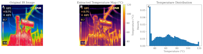
Figure 1: Temperature Visualization. (A) Original infrared (IR) thermographic image of the inspected high-voltage equipment showing the observed thermal pattern. (B) Extracted temperature map obtained from the thermographic image, illustrating the spatial distribution of surface temperatures and associated thermal gradients. (C) Temperature distribution histogram showing the frequency distribution of temperature values within the extracted temperature field. This figure demonstrates the conversion of a thermographic image into a quantitative temperature representation and summarizes the underlying temperature distribution used for subsequent model development and analysis. Abbreviations; IR = infrared. Please click here to view a larger version of this figure.

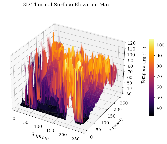
Figure 2: 3D thermal surface elevation representation of the temperature field. Three-dimensional visualization of the temperature distribution, where surface elevation corresponds to temperature magnitude and highlights localized thermal hotspots. Please click here to view a larger version of this figure.

Problem formulation

Let

 

denote the RGB infrared thermographic image, where H and W represent the spatial dimensions and C = 3 corresponds to the color channels associated with the rainbow thermal palette. Although the infrared image visually represents thermal information, it is not a direct numerical temperature matrix because the displayed colors depend on palette mapping, scaling, interpolation, and imaging conditions.

Let

 

denote the corresponding ground-truth temperature field obtained through radiometric calibration and temperature extraction from the infrared imaging system.

The learning objective is to approximate the mapping

where θ denotes the trainable parameters of the CNN and T̂ represents the predicted temperature field. The purpose of this supervised mapping is not simply to reproduce direct radiometric conversion, but to learn a spatially consistent temperature regression model from rendered thermographic images. Unlike direct pixel-wise color-to-temperature extraction, the CNN can exploit contextual thermal structure across neighbouring regions, reduce noise sensitivity, preserve hotspot characteristics, and generate smoother physically plausible temperature fields under the imposed diffusion constraints. The baseline objective function minimizes the pixel-wise regression error between the predicted and calibrated temperature fields:

where T_ij and T̂_ij denote the ground-truth and predicted temperatures at pixel location (i, j), respectively. Accordingly, the framework should be interpreted as a physics-regularized thermographic regression model rather than a replacement for direct radiometric calibration.

Infrared image acquisition conditions
Infrared thermographic images were acquired using a FLIR thermal imaging camera under outdoor substation operating conditions. The dataset consisted of RGB thermographic images with a spatial resolution of 640 × 480 pixels, recorded using the FLIR rainbow color palette. Each image included an embedded thermal scale bar indicating the temperature range associated with the acquisition frame. The thermographic inspection covered multiple categories of high-voltage equipment, including transformers, bushings, insulators, connectors, and terminal structures. Images were captured during normal operating conditions to include both standard thermal behavior and localized hotspot patterns relevant to condition monitoring applications. Image acquisition was performed from practical inspection viewpoints typically used in field thermography. The camera orientation and viewing angle varied depending on equipment accessibility and substation layout. Thermal images were visually screened to ensure that the target equipment remained clearly observable and that the hotspot regions were distinguishable from the background. The dataset was organized into labeled folders according to equipment category and thermal condition. Prior to model development, the images were segmented and resized into a consistent spatial format for temperature-field extraction and CNN training. The thermographic images contain thermal distributions suitable for computer vision and deep learning studies involving hotspot detection, fault identification, anomaly localization, and temperature-field prediction. In the present work, the thermal profiles extracted from the infrared images were used for physics-constrained temperature estimation and uncertainty-aware thermal assessment.

Thermographic dataset and data partitioning
The dataset used in this study consisted of 174 infrared thermographic images acquired from high-voltage substation equipment using a FLIR thermal imaging system¹⁵. The dataset included multiple types of power-system components, including transformers, bushings, insulators, connectors, and high-voltage terminal structures operating under practical outdoor conditions. Each thermographic image was converted into a spatial temperature field using the radiometric information provided by the infrared camera. The dataset contains thermal variations ranging from normal operating conditions to localized hotspot regions associated with elevated thermal stress. The data were divided into training, validation, and test subsets with a 70:15:15 split, yielding 121, 26, and 27 images, respectively. The partitioning was performed at the image level because the dataset consisted of independently captured thermographic scenes collected under varying operating conditions and viewpoints. Care was taken to avoid near-duplicate frames across subsets in order to reduce data leakage risk and improve evaluation fairness. All images were resized to a uniform spatial resolution prior to training. Temperature normalization was applied to stabilize optimization while preserving relative thermal gradients and hotspot characteristics important for condition assessment.

Baseline CNN architecture
A fully convolutional encoder–decoder regression architecture was adopted to preserve spatial resolution during temperature-field prediction from infrared thermographic images. All input infrared images were resized to a uniform resolution of 256 × 256 × 3 prior to training. The encoder section consisted of four convolutional blocks with progressively increasing feature depth. Each block contained a 3 × 3 convolution layer followed by batch normalization and ReLU activation. Spatial downsampling was performed using strided convolutions rather than max pooling to better preserve localized thermal structures and hotspot information. The encoder channel progression was:

32 → 64 → 128 → 256

The decoder section reconstructed the spatial temperature field using transposed convolution layers for upsampling with the reverse feature progression:

256 → 128 → 64 → 32

Each decoder block similarly employed transposed convolution, batch normalization, and ReLU activation. A final 1 × 1 convolution layer generated the predicted single-channel temperature map:
T̂ ∈ ℝ^256×256

The network therefore outputs a full-resolution spatial temperature field corresponding to the infrared input image. To support uncertainty quantification, dropout layers with probability p = 0.2 were inserted near the bottleneck and decoder stages. During inference, dropout remained active to enable Monte Carlo sampling for predictive uncertainty estimation. All convolutional weights were initialized using He-normal initialization, while bias terms were initialized to zero. The model was trained using the Adam optimizer with an initial learning rate of 1 × 10⁻³, batch size of 8, and weight decay of 1 × 10⁻⁵. Training was performed for 100 epochs using cosine learning-rate decay and early stopping based on validation RMSE.

The baseline objective function is defined as:

     

where L_data denotes the pixel-wise mean squared error between predicted and ground-truth temperature fields.
Performance was evaluated using: R², RMSE, and MAE.

Although the baseline CNN successfully captured the overall thermal structure and hotspot distribution, it occasionally produced non-physical artifacts in low-gradient regions and slight oversmoothing near sharp thermal boundaries. These limitations motivated the introduction of diffusion-based physics regularization in the subsequent model formulation.

Physics-constrained learning via diffusion
Governing heat equation
To enforce thermal consistency in the predicted temperature field, a diffusion-based physics prior was incorporated into the heat equation. Under quasi-steady conditions, the surface temperature approximately satisfies

   

where T denotes temperature, α is thermal diffusivity, and S represents local heat generation. Since the available thermographic samples are single inspection snapshots rather than time-resolved sequences, the temporal derivative cannot be directly evaluated. Accordingly, the model assumes local quasi-steady conduction and enforces

     

away from active heating regions.

The 2D Laplacian was discretized using the standard finite-difference stencil:
      

The physics residual was then computed over the predicted temperature map as

     

To avoid ambiguity at the image boundaries, the Laplacian residual was evaluated only on valid interior pixels, where all neighboring values required by the stencil are available. No explicit masking was applied to hotspot regions, since the objective of the physics term was to regularize the full spatial field rather than suppress thermally active zones. The hotspot structure was therefore learned through the data term, while the Laplacian penalty encouraged diffusion-consistent smoothness across the predicted map.

The final objective function combined the data loss and the physics loss as 

     

where λ_phys controls the strength of the physics regularization. In the ablation study, λ_phys ∈ {0, 10⁻⁴, 10⁻³, 10⁻², 10⁻¹} was examined to assess the effect of increasing physical constraint strength. Moderate values improved generalization, whereas overly strong weighting tended to oversmooth sharp hotspot gradients. This behavior is consistent with the thermal structures observed in the infrared images, where physically smooth regions coexist with localized high-temperature concentrations.

It should be emphasized that the steady-state diffusion formulation used in this work is not intended to represent the complete heat-transfer mechanism governing hotspot formation in high-voltage equipment. In practice, localized overheating arises from internal heat-generation processes such as Joule heating, contact resistance, and insulation degradation. Because the available dataset consists of snapshot thermographic images without temporal information or source measurements, the diffusion constraint is employed as a physics-inspired spatial regularization term. Its role is to encourage locally smooth, physically plausible temperature fields while allowing the hotspot characteristics to be learned from the data. Therefore, the diffusion prior should be interpreted as a spatial smoothness constraint rather than a comprehensive model of the underlying thermal physics.

Learnable thermal diffusivity and source-term augmentation
To improve physical interpretability, the effective thermal diffusivity was treated as a trainable scalar parameter. Let T̂(x, y) denote the predicted temperature field and let α > 0 denote the learnable thermal diffusivity. To enforce positivity, α was parameterized through an unconstrained variable β as

   

In this formulation, the physics prior was written in terms of an effective residual forcing field R(x, y), where R(x, y) represents the local departure from pure diffusion induced by unmodeled heating effects. The adaptive-diffusivity relation is therefore expressed as

     

Here, ∇²T̂(x, y) is the Laplacian of the predicted temperature field, and R(x, y) is the effective residual source term inferred implicitly from the thermographic data. Because the available samples are snapshot images rather than time-resolved thermal sequences, R(x, y) is not separately supervised and serves only as a latent physics quantity during optimization. The corresponding physics loss was defined as

   

For the source-term augmented experiment, an auxiliary CNN head was added to estimate a spatial source map Ŝ(x, y). In this case, Ŝ(x, y) represents the predicted local heat-generation field, and the governing relation becomes

   

The source head was attached to the encoder bottleneck and consisted of a small convolutional branch that mapped shared latent features to a single-channel output map Ŝ(x, y). No ground-truth source labels were available; therefore, Ŝ(x, y) was learned only through the joint objective

   

where L_data is the temperature regression loss, λ_phys controls the diffusion constraint, and λ_s regularizes the source prediction to discourage trivial high-magnitude source maps. In the snapshot-based setting considered here, the source-term formulation remained underdetermined and did not improve prediction accuracy.

Monte Carlo dropout for uncertainty quantification
To estimate epistemic uncertainty in the predicted temperature field, Monte Carlo dropout was applied during inference. Dropout layers with a rate of 0.2 were placed after the bottleneck block and within the decoder stages of the CNN. During testing, these dropout layers were kept active, and 30 stochastic forward passes were performed for each infrared image. For the k-th stochastic pass, the predicted temperature field is denoted by

   

where X is the input infrared image and θ_k represents the sampled network parameters induced by dropout. The predictive mean was computed as

   

and the pixel-wise predictive variance was obtained as

   

with K = 30. The resulting variance map was used to identify spatial regions with lower predictive confidence. Because ground-truth uncertainty labels are not available for thermographic regression, uncertainty was evaluated using pixel-wise variance maps and summary statistics computed over hotspot and background regions, rather than calibration-based metrics. The quantitative analysis showed that the mean predictive standard deviation was 13.046 °C, while the hotspot region exhibited a higher standard deviation of 15.934 °C compared with 12.743 °C in the background region. This corresponds to an approximately 25% increase in uncertainty within hotspot areas relative to the background. These results indicate that the model expresses greater uncertainty near thermally complex regions, particularly around hotspot boundaries and steep temperature gradients, which is consistent with the structure observed in the thermal surface visualizations. The workflow is summarized in Figures 3 and 4 shows the overall CNN-based processing pipeline.

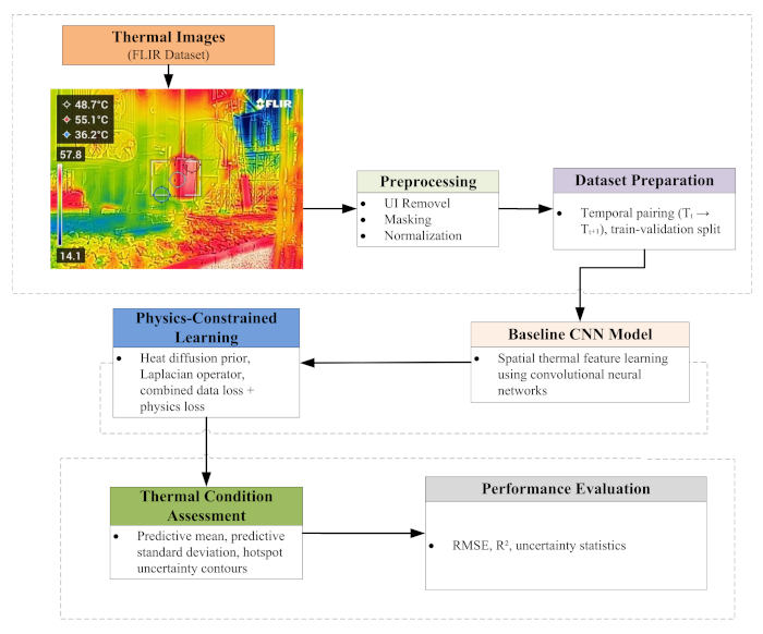
Figure 3: Workflow. Overview of the proposed methodology, including thermographic image acquisition, preprocessing, temperature-field extraction, CNN training, physics-constrained learning, and uncertainty quantification. Abbreviations; CNN = convolutional neural network. Please click here to view a larger version of this figure.

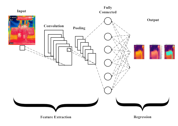
Figure 4: Overall CNN-based processing pipeline. Architecture of the proposed CNN framework showing the transformation of infrared thermographic images into spatial temperature-field predictions. Abbreviations; CNN = convolutional neural network. Please click here to view a larger version of this figure.

Results

This section evaluates the proposed physics-constrained deep learning framework using quantitative metrics and visual analysis. The results demonstrate how integrating diffusion-based physical constraints and uncertainty modeling influences predictive accuracy and thermal interpretability.

Performance comparison of model configurations
Table 1 shows the performance comparison of different model configurations. The baseline CNN achieved an RMSE of 12.345 °C...

Discussion

The present study investigated the integration of physics-based regularization and uncertainty-aware deep learning for thermal condition assessment of high-voltage power equipment using infrared thermographic imagery. The results show that embedding physical priors into CNN-based temperature prediction improves the robustness and physical consistency of the learned thermal fields relative to purely data-driven approaches. One of the most important findings is the role of the diffusion-based physics constraint in shaping ...

Materials

List of materials used in this article

Name	Company	Catalog Number	Comments
CUDA / cuDNN	NVIDIA	GPU acceleration for training	GTX 1080 Ti
Infrared thermographic camera	FLIR thermal imaging camera	Acquisition of high-voltage equipment thermograms	portable professional FLIR C5 Infrared camera at different times of the day and load conditions.
Jupyter Notebook / IDE	JupyterLab 4.2.0	Experiment development and analysis	Used in implementation
Matplotlib	Matplotlib Developers	Visualization of predictions, residual maps, and uncertainty maps	Used for figures and plots
NumPy	NumPy Developers	Numerical computing and array operations	Data preprocessing and tensor handling
OpenCV	OpenCV Foundation	Image loading, resizing, and basic preprocessing	Used for thermographic image handling
Python	Python Software Foundation	Main programming environment	Version used for all experiments
PyTorch	PyTorch Foundation	CNN training, physics-constrained learning, and Monte Carlo dropout	Used for implementation of the regression network
Scikit-learn	scikit-learn Developers	Metric computation and train/validation/test evaluation	Used for (R^2), RMSE, and MAE
SciPy	SciPy Developers	Supporting numerical routines	Used in preprocessing or analysis
Thermographic dataset	In-house field inspection dataset	Source of 174 infrared images for model development	Images organized in labeled folders
Workstation / GPU computing system	GTX 1080 Ti	Model training and inference	12 GB RAM,  GTX 1080 Ti , and Windows 11 OS